Development of a Framework for a Functional-Structural Seagrass

Transplantation Simulation using GAMA Platform

Therese Anne Rollan

, Ariel Blanco

and Edgardo Macatulad

Department of Geodetic Engineering, University of the Philippines, Diliman, Quezon City, Philippines

Keywords: Agent-based Modelling, Geographic Information System, Seagrass Growth Simulation, Seagrass

Transplantation, Plant Growth Modelling, Functional-Structural Approach, GAMA Platform.

Abstract: A massive decrease in seagrass coverage in the Philippines has been observed in the past several years due to

coastal eutrophication and typhoons. It is key to observe the changes and probable damage in seagrass habitat

and develop a way to scientifically back up recovery strategies such as transplantation to increase the

probability of rehabilitation success. This study describes the framework development of a transplantation

scenario evaluation tool that performs Thalassia hemprichii growth simulation within an uproot site in

Palawan as a case study. The growth parameters used include shoot leaf area, spacer length, plastochrone

interval, and life expectancy, and horizontal apex density. Base scenario and three scenarios with varying

combinations of transplantation density and distribution were applied to the three 4 x 4 grid plots with 24 x

24 cm cell size from classified drone imagery. Results show that transplantation distribution has a greater

weight than density with respect to the percent cover responses. Based on the mean and standard deviation of

percent cover responses, scenario 1 having 4 transplants with 24 cm intervals is the most suitable for plots 1

and 2, while scenario 2 having 8 transplants (2 per cell) with 24 cm intervals for plot 3.

1 INTRODUCTION

Seagrasses are clonal flowering plants that share the

same architecture (Marba, Duarte, Alexandria, &

Cabaco, 2004), submerged in shallow marine waters

(Florida Fish and Wildlife Conservation

Commission, n.d.), usually located on semi-enclosed

lagoons and along coastlines, and co-existing with

intertidal mangroves and corals (Fortes M. D., A

Review: Biodiversity, Distribution and Conservation

of Philippine Seagrasses, 2013). They play an

important role in providing food and shelter for

various marine species (Duarte & Chiscano, 1999;

Heiss, Smith, & Probert, 2000), stabilizing the sea

bottom (Borowitzka, Lavery, & van Keulen, 2006),

maintaining water quality, supporting the livelihood

of local economies and holds around 12% of the total

ocean carbon stock (UNEP, 2004). Among the

thriving species of seagrass in the Philippines,

Thalassia hemprichii (T. hemprichii) is one of the

dominant ones that exhibits horizontal expansion

https://orcid.org/0000-0002-8436-8165

https://orcid.org/0000-0002-0489-9979

https://orcid.org/0000-0001-7977-2932

typically in a span of approximately 5 to 11 days

(Lopez, Unpublished; Vermaat, et al., 1995).

A massive decrease in seagrass coverage in the

Philippines has been observed in the past several

years. It is key to monitor the changes and probable

damage and develop a way to scientifically justify

recovery strategies such as transplantation to increase

the probability of rehabilitation success. This study

aims to develop a framework for simulating seagrass

recovery in order to increase the certainty of

transplantation spatial strategy success in order to

help a seagrass meadow recover from a typhoon

damage. It will assist local communities, government

authorities, and researchers to formulate effective

strategies not only for seagrass recovery but also for

its rehabilitation and conservation.

The main question is how can a simulation be

applied to possibly increase the certainty of

transplantation spatial strategy success and help a

seagrass meadow recover from a typhoon damage.

The framework aims to answer the following:

248

Rollan, T., Blanco, A. and Macatulad, E.

Development of a Framework for a Functional-Structural Seagrass Transplantation Simulation using GAMA Platform.

DOI: 10.5220/0010520502480255

In Proceedings of the 11th International Conference on Simulation and Modeling Methodologies, Technologies and Applications (SIMULTECH 2021), pages 248-255

ISBN: 978-989-758-528-9

 What are the primary datasets needed?

 What steps must be done to run a seagrass

transplantation simulation?

From the results of the transplantation simulation

scenarios, the following are the questions aimed to be

answered:

 What are the corresponding seagrass percent

cover tracks?

 What metrics can be used to describe the

behavior of these tracks?

 From the scenario factors considered, which of

them are statistically significant? Which have

greater bearing on the metrics considered?

2 LITERATURE REVIEW

2.1 Seagrasses

2.1.1 Overview

Seagrasses belong to plants producing flowers known

as angiosperms, evolved to thrive in marine waters

and typically have ribbon-like, grassy leaves

(McKenzie, 2008) with its general structure divided

into above-ground including leaf, blade and stem and

below-ground consisting of rhizome (horizontal) and

root (El Shaffai, 2016). They follow a clonal

mechanism called vegetation proliferation sharing

similar architecture but with varying plant size and

growth rate across species (Marba, Duarte,

Alexandria, & Cabaco, 2004).

2.1.2 Disturbances, Rehabilitation,

Transplantation and Recovery

Since some are located in deep areas, light becomes

crucial and exposure to disturbances becomes higher

(Greve & Binzer). These disturbances are caused by

anthropogenic activities and natural phenomena

(Short & Wyllie-Echeverria, Natural and human-

induced disturbances of seagrass, 1996). Oil spill

incidents were reported in the Philippines in 1987

(Fortes M. D., 1991), Puerto Rico in 1962 and

California in 1969 (Zieman, Orth, Phillips, Thayer, &

Thorhaug, 1984). In the U.S., a continuous decrease

in percent cover was observed from 2003 to 2008

including a dramatic decline by 2006 due to a storm

wave (Buchanan, 2009). In Banate Bay, Philippines,

seagrasses were uprooted by typhoon Haiyan (The

Philippine Star, 2016). Although, their response to

environmental and population changes are species-

specific (Marba, Duarte, Alexandria, & Cabaco,

2004), as observed as well by Duarte et al. (1987).

Their recovery relies on vegetative growth, regrowth

from fragments of transported plants, and recovery

from seeds (Vanderklift, et al., 2016). Rollon et al.

(1998) showed that the projected duration of post-

disturbance recovery ranges from 2 to 10 years in full

recovery both for artificially created gaps of 0.25

sq.m. Another study observed gradual recovery

within 2 to 6 years after a cyclone and consequent

flood (Campbell & McKenzie, 2004).

2.1.3 Thalassia Hemprichii

Genus Thalassia consists of two species, T.

testudinum and T. hemprichii, a.k.a. “twin species”

because they can only be distinguished through the

counts and dimensions of the styles and stamens of

their flowers appearance-wise (van Tussenbroek, et

al., 2006). Both grow in highly organized and rigid

pattern which primarily depends on the active tip of

the horizontal (h.) rhizomes called apical meristem or

apex for expansion (Tomlinson, 1974). To survive,

vertical rhizomes utilize surrounding resources,

deploying leaves and roots at the same (Hemminga &

Duarte, 2000). T. hemprichii is a commonly

widespread species and is considered to be stable

despite threats and disturbances (Short, et al., 2010).

In the Philippines, it commonly thrives on mud-coral-

sand or coarse coral-sand substrates and grows up to

6 meters deep (Menez, Phillips, & Calumpong, 1983).

2.2 Agent-based Modeling

2.2.1 Overview

Agent-Based Modeling (ABM) utilizes objects called

agents possessing attributes and behaviors, and

playing specified roles in the model through specified

rules and constraints. Its advantages include capturing

of emergent phenomena, provision of a natural

environment for the study of certain systems, and

flexibility (de Smith, Goodchild, & Longley, 2018).

Moreover, it is capable of handling high

heterogeneity in characteristics, interactions between

agents and environments, and their dynamics,

feedbacks and adaptation (Auchincloss & Garcia,

2015). In the past decades, this method has already

been widely used in different fields. However, due to

lack of awareness in the significant importance of

seagrass, studies on seagrass growth simulation

employing this method is still relatively sparse.

Development of a Framework for a Functional-Structural Seagrass Transplantation Simulation using GAMA Platform

249

2.2.2 Gama Platform

GIS Agent-based Modeling Architecture Platform

(GAMA) is an open-source environment that

combines agent-based simulations with spatial

applications (Grignard, et al., 2013). It uses its own

programming language GAML (GAMA Modeling

Language) coded in Java which makes them similar

in syntax and structure (GAML, 2018). In

conjunction with the visualization, instantaneous

statistics of the agents and the simulation can be

displayed using graphs.

2.2.3 Functional-Structural Plant Model

One approach is Cellular Automata which treats a

seagrass plot as a grid having each grid cell a value

representing percent cover or biomass (Marsili-

Libelli & Giusti, 2004). However, this can be quite a

generalized approach if the target is to visualize and

analyze the components in detail. To achieve these,

ABM must be employed wherein Functional-

Structural Plant Model (FSPM) can be applied. It is

suitable in simulating seagrass growth because the

plant is modelled in a much finer detail (Godin &

Sinoquet, 2005) such as its roots, leaves and branches

to simulate the higher-level outcomes (Dejong, Da

Silva, Vos, & Escobar-Gutiérrez, 2011). Related

studies include the works of Sintes et al. (2005),

Renton et al. (2011), and Whitehead et al. (2018).

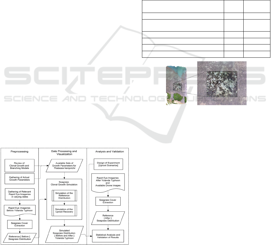
3 MATERIALS AND METHODS

This research is divided into three main procedures

namely 1) Pre-processing, 2) Data Processing and

Visualization, and 3) Analysis and Validation.

Figure 1: This is the research workflow for the development

of the seagrass transplantation simulation framework.

3.1 Pre-processing

This stage involves literature review, gathering of

growth parameters (Table 1), gathering of site

datasets shown in Figure 2, seagrass percent cover

extraction using Mixed-Tuned Matched Filtering

(MTMF) method in ENVI software, and

identification of three random plots within the

blowout scenarios that will represent three plots or the

number of repetitions of the transplantation

simulation runs.

Table 1: T. hemprichii parameters used in the developed

transplantation simulation are summarized below as

adapted and derived from the work of Vermaat, et al.,

(1995), and from Ms. Rose Lopez and Dr. Rene Rollon.

Parameter Value Standard

deviation

Shoot leaf area (sq.cm, single-sided) 26.56 0.02

Shoot spacing along rhizome

(spacer length, cm)

6.77 2.90

Shoot

lastochrone interval (PI, days) 4.03 0.34

Shoot life expectancy (days) 229 17

Rhizome apex density per sq. m 58 -

Rhizome life ex

ectanc

(years) 4 -

Figure 2: This is a drone imagery captured by a project team

under the IAMBlueCECAM Program on September 2017

on a seagrass blowout site in Palawan, Philippines.

In the seagrass extraction, two drone image spatial

resolutions were used: the original resolution 6 cm and

the resampled 24 cm. To obtain the grids, ArcMap

Fishnet tool was used to generate a 24 x 24-cm grid

resolution. To determine the three random plots within

the blowout that will represent three transplantation

simulation repetitions, ArcMap Create Random Points

tool was used. The extent for the previously generated

grid served as a coverage constraint in order to ensure

that the points will not fall outside the blowout site.

Minimum allowable distance from each of the points

was set to 20 meters to avoid them from being too close

to each other. The grid cell where these points fell into

are the upper left corner of the 4 x 4 grid, having cells

with dimensions 24 x 24 cm. In Figure 3, the

preparation for the input grids is demonstrated. Values

in percent are converted to their decimal format and

used in the transplantation simulation as comma-

separated (csv) files.

SIMULTECH 2021 - 11th International Conference on Simulation and Modeling Methodologies, Technologies and Applications

250

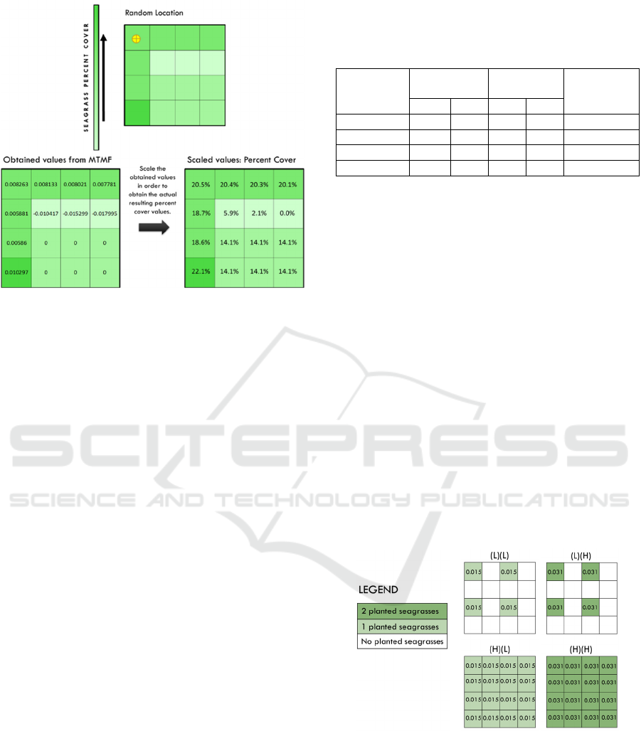
Figure 3: Obtaining the input percent cover grids from the

MTMF classification output and the randomly generated

locations: Illustrations above represent a single random plot

from a random location shown as yellow marker at the

upper leftmost cell of the 4 x 4 grid.

3.2 Data Processing and Visualization

In this stage, parameters in Table 1 and the extracted

seagrass percent cover for each plot are the input for

the seagrass transplantation simulation. Prior to the

simulation proper, the input csv files for each scenario

of the three random plots must be prepared.

Following Table 2, four scenarios of varying level

combinations for low and high of factors a) planting

distribution and b) planting density. Low level (L) for

the planting distribution means wide intervals

between plants and high level (H) corresponds to

closer intervals. On the other hand, L for planting

density denotes 1 plant per grid cell of 24 x 24 cm and

H indicates 2 plants per cell. There will be five

percent cover responses: Sum, Mean, Standard

Deviation, Minimum, and Number of Extreme Drops.

To represent these scenarios as input files for the

transplantation simulation, corresponding template

for each were created by computing their density (per

grid cell of size 24 x 24 cm) contributions as shown

below by the equations 2 and 3. These templates are

grids with values having the dimensions with the

plots. The shoot leaf area from Table 1 cannot be

directly used since it assumes that the leaf is

completely horizontal, facing the drone upon imagery

capture. Due to water depth and current, seagrass

leaves are angled, if not upright. Thus, we use a

reduction factor which in this case is 1/3 according to

our consultation with Dr. Rollon as demonstrated in

equation 1.

Table 2: This table illustrates the Design of Experiments

(DOE) for the four seagrass transplantation scenarios with

varying level combinations for low and high of factors a)

planting distribution and b) planting density.

Scenario

Planting

Distribution

Planting

Densit

Percent

Cover

Response

LHL H

1× × R1

2× × R2

3×× R3

4× × R4

Derived shoot leaf area per plant (sq.cm.) =

(1/3)26.56 = 8.85

(1)

Derived shoot leaf area density for Planting

Density (L) = (1 plant x 8.85)/(24 x 24) = 0.015

(2)

Derived shoot leaf area density for Planting

Density (H) = (2 plants x 8.85)/(24 x 24) =

0.031

(3)

In Figure 4, L stands for low factor level and H

the high factor level. The first letter denotes the level

of factor a) planting distribution while the second

letter for b) planting density such that (L)(L) stands

for transplantation scenario #1 from Table 2. These

scenario grids are added to each of the three random

plots creating five transplantation simulation runs for

each namely: i) scenario 0 - base scenario or the actual

percent cover based on the drone-obtained imagery,

and ii) scenario 1 to 4. They are then converted to csv

files as inputs for the reference meadow with percent

cover values.

Figure 4: Seagrass transplantation scenario templates with

the computed values of the percent cover contribution of the

seagrasses to be planted.

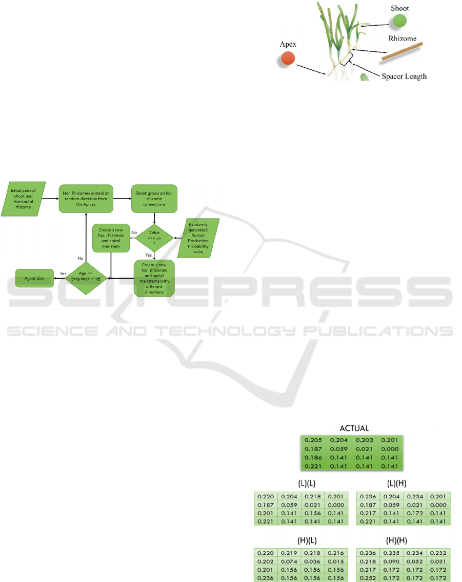
Figure 5 describes the flow of the simulation

starting from the initial pairs of h. rhizome and shoot.

Due to the lack of firm literary basis for the initial

seagrass plants per unit area that may populate and

turn into a meadow, the chosen ratio between the

number of initial pairs to the percent cover is 1:10.

Development of a Framework for a Functional-Structural Seagrass Transplantation Simulation using GAMA Platform

251

Though this is a part of the assumptions, this ratio is

still reasonable since it partially and relatively

describes the reference meadow.

Every transplantation simulation cycle, new h.

rhizomes will emerge from the locations of the apices

in a random direction. Randomized runner production

probability determines whether there will be one or

two emerging rhizomes. If the probability is ≤ 10%, a

runner is produced and two new h. rhizomes will be

created. From the current apex agents, shoot agents

will grow on the next cycle. In addition, old apex

agents will die (disappear in the transplantation

simulation) and new apex agents will grow from the

tips of the new h. rhizomes. Previously created shoot

and h. rhizome agents will remain until they reach the

maximum age imposed. Every cycle, agent count and

percent cover value are logged and graphed.

Figure 5: Seagrass Transplantation Simulation

Implementation Workflow.

The geo-simulation uses agents to represent the

main components of seagrass growth, namely the

apical meristem or apex, the h. rhizome and the shoot

as illustrated in Figure 6. Apex (apical meristem) is

represented as red circle, shoot as green circle and h.

rhizome as brown line. The growing tip or meristem

of a shoot is represented by the Apex which can

produce new rhizomes and apices. Shoots grow at the

nodes of h. rhizomes. Since the simulation is limited

to two-dimensional top view visualization, shoots are

simplified and represented as green circles.

The transplantation simulation parameters used

include apex density, plastochrone interval (denoted

by P.I.; number of days within which h. rhizome is

produced), horizontal elongation rate, branching rate,

h. rhizomes between shoots, shoot spacing along

rhizome and median maximum age of shoot and

rhizome. The time step used is 4.03 ± 0.34 days which

represents the duration of rhizome growth and a

threshold of 58 apices denoting the maximum number

in an almost 1 sqm. plot. Simulation run starts from

randomly distributed pairs of apex and rhizome over

a specified relatively small plot and grow into

meadows covering a spatial distribution with respect

to a corresponding reference seagrass percent cover.

Figure 6: A simplified top view representations of seagrass

agents T.hemprichii with its photo adapted from

(SeagrassWatch.org).

3.3 Analysis

The final stage of the methodology is the analysis in

which the graphs for each of the plot’s scenario result

was observed and the trends of the values are

discussed and explained. Using Design Expert

software, the analysis of variance (ANOVA) and

interaction among factor levels were examined. This

will show if the factors and their levels are significant.

4 RESULTS AND DISCUSSION

4.1 Reference Seagrass Meadows

Figure 7 summarizes the actual or the reference

percent cover plots (scenario 0) and their four

scenarios obtained by taking into account the

combinations of the levels of the two factors in the

DOE table (Table 2). Each row of the said figure

represents a repetition (or the plots as discussed in

Section 3.1). All of these are formatted as csv files

and were used as inputs in the transplantation

simulation.

Figure 7: Percent cover grid per plot for the actual values

and the scenario factor levels.

SIMULTECH 2021 - 11th International Conference on Simulation and Modeling Methodologies, Technologies and Applications

252

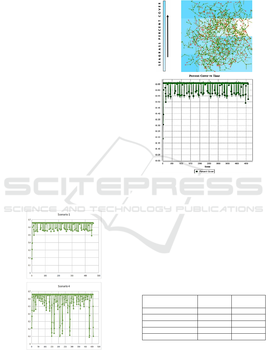
4.2 Seagrass Transplantation

Simulation Results

In the transplantation simulation, four quantities were

kept track over time (1 transplantation simulation

cycle = 1 P.I. from Table 1) for a total span of 5 years

namely percent cover, and shoot, horizontal rhizome

and apical meristem counts. For each plot scenario,

the maximum potential seagrass percent cover is

66%. This is due to the agent constraints which are

imposed based on the maximum number of apical

meristems per plot and the agents’ respective

lifespans according to Vermaat, et. al. (1995) and Dr.

Rollon. Since percent cover is calculated from an

orthogonal viewpoint wherein only the shoots are

visible, the percent cover progression can be derived

from the trend of the shoots. Abrupt percent cover

drops result from a number of shoot agents that occur

simultaneously which in turn dies simultaneously.

Hence, extreme percent cover drops do not

necessarily mean that the seagrass meadow will

continuously thin.

In choosing the best planting scenario, standard

deviation and mean were considered. Standard

deviation accounts for the fluctuations of the percent

cover values. Hence, the best planting scenario per

study plot is characterized by low standard deviation

and high mean. Figure 8 illustrates the comparison

between two scenarios. Apparently, scenario 1 is

better than scenario 4 in this case (Figure 9).

Figure 8: This figure compares two scenarios (1 and 4) in

order to choose the better planting scenario. Note that the

comparisons are among the four scenarios per plot.

Figure 9: This shows the transplantation simulation results

of Plot 1 with Scenario 1 as the best scenario.

4.3 DOE Results

The importance of the factors with respect to the

responses by observing their relative significance

through their corresponding weights summarized in

Table 3. Sum and Mean are the most and least

significant percent cover response, respectively, both

to the planting distribution and planting density.

Furthermore, the factors were found to be

independent of each other a factor can be examined

separately without considering the other.

Table 3: This table contains the weight of each percent

cover responses shown.

Percent Cover

Res

onse

Planting

Distribution

Planting

Densit

Sum 0.993 0.548

Mean 0.002 0.001

Standar

Dev. 0.005 0.003

Minimum 0.009 0.012

No. of Extreme Dro

s 0.750 0.375

The DOE table as shown in Table 2 was

completed with five percent cover responses sum,

mean, standard deviation, minimum, and number of

extreme percent cover drops. It was observed that the

Development of a Framework for a Functional-Structural Seagrass Transplantation Simulation using GAMA Platform

253

model factors planting distribution and planting

density, and levels in this case study are not

significant using 95% confidence level with respect

to the previously enumerated responses. However,

based on how seagrass transplantation are practically

planned and carried out, these factors are still viewed

as worthy of research attention. It is just unfortunate

that this result may be due to a number of study

limitations brought about by the short duration and

lack of fieldwork budget of the project under which

this study was undertaken. These limitations include

the lack of field-obtained datasets such as drone

images in varying dates which can facilitate a

formulation of a sophisticated calibration and

validation procedure. Another is the lack of powerful

computers to simulate larger seagrass plots in longer

period. Nonetheless, these can serve as areas of

improvement for future researchers.

5 CONCLUSIONS AND

RECOMMENDATIONS

The study was able to develop and demonstrate a

framework for seagrass transplantation simulation.

The two factors planting distribution and planting

density appeared to be insignificant in the setup of

this study due to the presented limitations. However,

the importance (weight) of the factors with respect to

the responses can be observed based on the

coefficients derive from the DOE analysis. Majority

of the responses show that planting distribution has a

greater weight than planting density. Mean and

standard deviation were used to determine which

scenario will fit given the initial percent cover of a

plot -- Scenario 1 having 4 plants with 24 cm intervals

for Plots 1 and 2, while Scenario 2 having 8 plants (2

plants per grid cell) with 24 cm intervals for Plot 3.

Visualization techniques such 3D view of

seagrass agents closer to their real appearances can be

used in order to make non-technical persons

understand more easily the simulation outcomes.

Furthermore, a stand-alone software with more user-

friendly interface can be developed for government

and academic purposes. These future programs must

be optimized for usage efficiency to account for

machine capability limitations.

For the validation, it is highly encouraged to use

imageries of the same resolution as the reference

imagery. One method is to extract and compare

percent covers from the “after the simulation date”

imageries and compare them to the simulation percent

cover outcome.

ACKNOWLEDGEMENTS

This work is funded by the Department of Science

and Technology, Philippine Council for Industry,

Energy and Engineering Technology Research and

Development with Project No. 04041, 2018.

REFERENCES

Auchincloss, A., & Garcia, L. (2015, November). Brief

introductory guide to agent-based modeling and an

illustration from urban health research. Cad Saude

Publication, 65–78.

Borowitzka, M., Lavery, P., & van Keulen, M. (2006).

Epiphytes of seagrasses. In A. Larkum, R. Orth, & C.

Duarte, Seagrasses: biology, ecology and conservation

(pp. 441-461). the Netherlands: Springer.

Buchanan, S. W. (2009). Cape Cod National Shore

Resource Brief: Seagrass Monitoring. U.S. Department

of the Interior - National Park Service.

Campbell, S., & McKenzie, L. (2004). Flood related loss

and recovery of intertidal seagrass meadows in southern

Queensland, Australia. Estuar. Coast. Shelf Sci. 60,

477-490. Retrieved from http://refhub.elsevier.com/

S0025-326X(17)30741-5/rf0060

de Smith, M., Goodchild, M., & Longley, P. (2018).

Geospatial Analysis: A Comprehensive Guide to

Principles Techniques and Software Tools 6th Edition.

UK: The Winchelsea Press.

Dejong, T., Da Silva, D., Vos, J., & Escobar-Gutiérrez, A.

(2011). Using functional–structural plant models to

study, understand and integrate plant development and

ecophysiology. Annals of Botany 108, 987-989.

Duarte , C., & Chiscano, C. (1999). Seagrass biomass and

production: a reassessment. Aquatic Botany 65, 159-

174.

Duarte, C. M., & Kalff, J. (1987). Weight-density

relationships in submerged aquatic plants: the

importance of light and plant geometry. Oecologia,

72(4), 612-617.

El Shaffai, A. (2016). Field Guide to Seagrasses of the Red

Sea.

Florida Fish and Wildlife Conservation Commission. (n.d.).

Importance of Seagrass. Retrieved from Florida Fish

and Wildlife Conservation Commission Web site.

Fortes, M. D. (1991). Seagrass-mangrove ecosystems

management: a key to marine coastal conservation in

the ASEAN region. Marine Pollution Bulletin 22, 113-

116.

Fortes, M. D. (2013). A Review: Biodiversity, Distribution

and Conservation of Philippine Seagrasses. Philippine

Journal of Science 142, 95-111.

Fortes, M. D., Go, G. A., Bolisay, K., Nakaoka, M., Uy, W.

H., Lopez, M., Edralin, M. (2012). Seagrass response to

mariculture-induced physico-chemical gradients in

Bolinao, northwestern Philippines. 12th International

Coral Reef Symposium. Cairns, Australia.

SIMULTECH 2021 - 11th International Conference on Simulation and Modeling Methodologies, Technologies and Applications

254

GAML. (2018, September 8). Retrieved from GAMA

Platform Github Web site: https://gama-

platform.github.io/wiki/GamlLanguage

Godin, C., & Sinoquet, H. (2005). Functional-structural

plant modelling. New Phytologist 166, 705-708.

Greve, T. M., & Binzer, T. (n.d.). Chapter 4: Which factors

regulate seagrass growth and distribution?

Grignard, A., Taillandier, P., Gaudou, B., Vo, D., Huynh,

N., & Drogoul, A. (2013). GAMA 1.6: Advancing the

Art of Complex Agent-Based Modeling and

Simulation. In G. Boella, E. Elkind, B. Savarimuthu, F.

Dignum, & M. Purvis, PRIMA 2013: Principles and

Practice of Multi-Agent Systems. PRIMA 2013. Lecture

Notes in Computer Science, vol 8291 (pp. 117-131).

Berlin, Heidelberg: Springer. Retrieved from GAMA

Platform Homepage: https://gama-platform.github.io/

Heiss, W., Smith, A., & Probert, P. (2000). Influence of the

small intertidal seagrass Zostera novazelandica on

linear water flow and sediment texture. New Zealand J

Mar Fresh 34, 689-694.

Hemminga, M., & Duarte, C. (2000). Seagrass Ecology.

Cambridge, UK: Cambridge University Press.

Jackson, E. L., Rowden, A. A., Attrill, M. J., Bossey, S. J.,

& Jones, M. B. (2001). The importance of seagrass beds

as a habitat for fishery species. Oceanography and

Marine Biology: An Annual Review, 269-303.

Retrieved from ResearchGate: https://www.research

gate.net/publication/236683422

Lopez, R. (Unpublished). Master Thesis (University of the

Philippines Marine Science Institute).

Marba, N., Duarte, C., Alexandria, A., & Cabaco, S. (2004).

Chapter 3: How do seagrass grow and spread?

Marsili-Libelli, S., & Giusti, E. (2004). Cellular Automata

Modelling of Seagrass in the Orbetello Lagoon. 9th

International Congress on Environmental Modelling

and Software. Provo, Utah: BYU ScholarsArchive.

McKenzie, L. (2008, Feb). Seagrass-Watch: Seagrass

Educators Handbook.

Menez, E., Phillips, R., & Calumpong, H. (1983).

Seagrasses in the Philippines. Washington:

Smithsonian Institution Press.

Renton, M., Airey, M., Cambridge, M., & Kendrick, G.

(2011). Modelling seagrass growth and development to

evaluate transplanting strategies for restoration. Annals

of Botany 108, 1213–1223.

Rollon, R., De Ruyter Van Steveninck, E., Van Vierssen,

W., & Fortes, M. (1998). Contrasting Recolonization

Strategies in Multi-Species Seagrass Meadows. Marine

Pollution Bulletin Vol. 37, Nos. 8-12, 450-459.

SeagrassWatch.org. (n.d.). ID_Seagrass Images. Retrieved

from SeagrassWatch.org: http://www.seagrass

watch.org/ID_Seagrass/images

Short, F., & Wyllie-Echeverria, S. (1996). Natural and

human-induced disturbances of seagrass.

Environmental Conservation, 17-27.

Short, F., Carruthers, T., Waycott, M., Kendrick, G.,

Fourqurean, J., Callabine, A., Dennison, W. (2010).

The IUCN Red List of Threatened Species. Retrieved

from Thalassia hemprichii: http://www.iucnredlist.org/

details/173364/0

Sintes, T., Marba, N., Duarte, C., & Kendrick, G. (2005).

Nonlinear processes in seagrass colonisation explained

by simple clonal growth rules. OIKOS 108, 165-175.

The Philippine Star. (2016, April 3). Pfizer supports young

scientists to save environment. PhilStar Global.

Tomlinson, P. (1974). Vegetative morphology and

meristem dependence—the foundation of productivity

in seagrasses. Aquaculture 4, 107-130.

UNEP. (2004). Seagrass in the South China Sea. Bangkok:

UNEP.

van Tussenbroek, B., Vonk, J., Stapel, J., Erftemeijer, P.,

Middelburg, J., & Zieman, J. (2006). The Biology of

Thalassia: Paradigms and Recent Advances in Research

. In A. W. al., Seagrasses: Biology, Ecology and

Conservation (pp. 409-439). Springer.

Vanderklift, M., Bearham, D., Haywood, M., McCallum,

R., McLaughlin, J., McMahon, K., Lavery, P. (2016).

Recovery mechanisms: understanding mechanisms of

seagrass recovery following disturbance. Report of

Theme 5 – Project 5.4 prepared for the Dredging

Science Node, Western Australian Marine Science

Institution. Perth, Western Australia: Western

Australian Marine Science Institution.

Vermaat, J. E., Agawin, N. S., Duarte, C. M., Fortes, M. D.,

Marba, N., & Uri, J. S. (1995). Meadow maintenance,

growth and productivity of a mixed Philippine seagrass

bed. Marine Ecology Progress Series, 215-225.

Whitehead, S., Cambridge, M., & Renton, M. (2018). A

functional–structural model of ephemeral seagrass

growth influenced by environment. Annals of Botany

121, 897–908.

Zieman, J., Orth, R., Phillips, R., Thayer, G., & Thorhaug,

A. (1984). The effects of oil on seagass ecosystems. In

J. Cairns, & A. Buikema, Recovery and restoration of

marine ecosystems (pp. 37-64). Stoneham,

Massachusetts, USA: Butterworth Publications.

Development of a Framework for a Functional-Structural Seagrass Transplantation Simulation using GAMA Platform

255