
Dynamics Modelling and Simulation of Super Truss Element based
on Non-linear Beam Element
Lingchong Gao, Xiaobing Dai, Michael Kleeberger and Johannes Fottner
Chair of Materials Handling, Material Flow, Logistics, Technical University of Munich, Boltzmannstrasse 15,
85748 Garching, Germany
Keywords: Non-Linear Dynamics, Mobile Crane, Lattice Boom, Model Reduction.
Abstract: A mobile crane equipped with a lattice boom system is widely used to lift the heavy load on construction sites.
Even though the lattice structure can provide strong support with limited mass, the inertia force of the lattice
boom is still not neglectable, so is the heavy lifting load. Therefore, the dynamic response of the lattice boom
is important but also time-consuming due to a large number of degrees of freedom. In engineering, the truss
beam is often simplified as a continuous beam, but because of the noncontinuity of the truss, this direct
modelling method cannot truly reflect the actual dynamics of the truss. In this paper, a detailed Super Truss
Element formulation for nonlinear truss elements is proposed to reduce the number of degrees of freedom.
The formulation uses nonlinear spatial Timoshenko Beam based on co-rotational coordinate and dynamic
condensation approach with three assumptions. After parameterizing the characteristics of the Super Truss
Element, a nonlinear method for the calculation of the mass matrix and force vector in a large displacement
and rotation is developed. A dynamic simulation of the spatial motion of the lattice boom crane is performed
and the results are analysed.
1 INTRODUCTION
Among the large number of cranes developed for
various tasks, mobile cranes are particularly flexible
in their application possibilities. Truck-mounted
cranes, mobile cranes, railway cranes, and crawler
cranes are different cranes equipped with a boom
system, their booms can be designed as telescopic or
truss booms. Compared with the continuous boom
structure, the crane with a truss boom has a higher
load capacity under the same mass due to the
optimization of its structure. It is suitable for lifting
tasks with special requirements for lifting height and
radius. It is mainly used for large-scale factory
construction, steel, and building construction.
(Kleeberger 1996)
The form of cranes is diverse and complex. In the
design process, simulation and proofreading for
different types of cranes under different load cases are
required, which causes many calculations. As a kind
of engineering machinery, mobile cranes need to lift
a large load and move. Considering the mass of the
hoisting cargo and the boom structure, dynamics
calculations should be done, especially for some
extreme conditions in the holistic capacity sheet. The
dynamic modeling of lattice boom becomes difficult
due to the unevenness of cross-section and a large
number of nodes and elements. Previously there are
mainly two modeling methods:
1. Modeling of each element of the lattice boom.
The model will be closer to the actual lattice boom,
but due to a large number of nodes, the overall model
has a large number of degrees of freedom (Günthner
und Kleeberger 1997). This decreases the solution
speed and efficiency.
2. Modeling the entire lattice boom with a
continuous flexible beam element. This method can
greatly reduce the number of degrees of freedom and
accelerate the calculation of the system, but without
the necessary theoretical basis, the accuracy of the
model will be decreased.
Therefore, a scientific reduction method that
accelerates the model calculation and makes the
number of degrees of freedom small is urgently
needed.
For truss boom, there is a static condensation
method, which condenses the stiffness and gravity of
the truss beam to the nodes on the end section. This
method is only suitable for the static reduction of
linear models (Kleeberger und Hübner 2006).
50
Gao, L., Dai, X., Kleeberger, M. and Fottner, J.
Dynamics Modelling and Simulation of Super Truss Element based on Non-linear Beam Element.
DOI: 10.5220/0010519700500061
In Proceedings of the 11th International Conference on Simulation and Modeling Methodologies, Technologies and Applications (SIMULTECH 2021), pages 50-61
ISBN: 978-989-758-528-9
Copyright
c
2021 by SCITEPRESS – Science and Technology Publications, Lda. All rights reserved

For dynamics reduction, the Craig-Bampton
method is often used. It converts the dynamic
equations from the time domain into the frequency
domain to obtain information such as the natural
frequency of the system (Koutsovasilis und
Beitelschmidt 2007). However, for nonlinear models,
it is very difficult to convert them to the frequency
domain (Kammer et al. 2015).
In this paper, a super truss element with only two
nodes is proposed based on three assumptions. Under
the premise that the total energy of the super truss
element is the same as the actual truss model, this
element can condense the mass matrix and force
vector of each flexible body, normally each pipe, in
the truss. Therefore, the number of degrees of
freedom of the entire truss can be reduced to 12 and
solving speed of dynamic calculation can be
increased.
2 SUPER TRUSS ELEMENT
2.1 Spatial Timoshenko Beam based on
Co-rotational Formulation
The large deformation of the truss element is caused
by the cumulative effects of small deformation from
elements in the truss. Therefore, we model each
element in the truss as a short beam with small linear
deformation. Here spatial Timoshenko beam based on
co-rotational formulation is used to model the beam
element of the truss.
2.1.1 Co-rotational Coordinate
The co-rotational coordinate describes the position of
the element without deformation. The deformation of
any point on the element is based on the co-rotational
coordinate.
The co-rotational coordinate 𝒒
can be defined by
the coordinates of the two ends of the element, where
the script “B” represents the co-rotational coordinate
system (base coordinate system), the script “e”
represents the element coordinate system and the
script “I” represents the inertial coordinate system.
𝒒
=
𝒓
𝝋
=𝒒
(
𝒒
)
𝒒
=
𝒒
𝒒
(1
)
where 𝒓
is the position vector of the origin point of
co-rotational coordinate expressed in inertial
coordinate, and 𝝋
is the Cartesian vector for co-
rotational coordinate.
The relationship between the generalized velocity
d𝒒
and acceleration d𝒒
of the co-rotational
coordinate and the generalized velocity d𝒒
and
acceleration d𝒒
of the end-point coordinates can be
expressed as
d𝒒
=
𝒓
𝝎
=𝑻
d𝒒
d𝒒
=𝑻
d𝒒
+𝑻
d𝒒
(2)
𝒒
, 𝑻
and 𝑻
can be determined according to the
definition of co-rotational coordinate system.
2.1.2 The Formulation of Deformation
According to the Timoshenko beam assumption, the
deformation of any point on the section 𝑐 is caused by
the centroid translational deformation of the section
𝒖
and the section rotational deformation 𝝍
. The
actual deformation of this point 𝒖
can be obtained
by the difference between the position vector before
deformation 𝒓
∗
and the after deformation 𝒓
,
𝒓
∗
=𝒓
+𝑹
(
𝒓
+𝒕
)
𝒓
=𝒓
+𝑹
𝒓
+𝒖
+𝑹
,
𝒕
(3)
where 𝒓
is the relative position of cross-section 𝑐
to the original point of co-rotational coordinate, and
𝒕
=
0𝑦
𝑧
is the relative position of any
point on cross-section 𝑐 to the sectional centre. 𝒓
and 𝒕
are constant for each cross-section.
Here we use the hypothesis of small rotational
deformation. The subscript “d” represents the
deformation coordinate. The rotation matrix 𝑹
,
for
axis-angle rotation vector 𝝍
can be written as:
𝑹
,
≈𝑰+ 𝝍
(4)
where 𝒂
represents the skew symmetric matrix of the
corresponding vector 𝒂.
Thus, the deformation can be approximated as
𝒖
=𝑹
(
𝒓
−𝒓
∗
)
≈𝒖
+𝝍
𝒕
(5)
The deformation coordinate of the end point
𝒒
,
can be expressed by the following formula
𝒖
=𝑹
(
𝒓
−𝒓
)
−𝒓
𝝍
=𝝍
𝑹
𝑹
= 𝝍
𝑹
,
𝒒
,
=
𝒖
𝝍
𝒖
𝝍
(6)
Dynamics Modelling and Simulation of Super Truss Element based on Non-linear Beam Element
51

The velocity and acceleration of the deformation
at the end point can be expressed by element
coordinate.
d𝒒
,
=𝑻
,
d𝒒
=
𝒖
𝝕
𝒖
𝝕
(7
)
d𝒒
,
=𝑻
,
d𝒒
+𝑻
,
d𝒒
(8
)
where 𝝕
represent the angular velocity of the
angular deformation 𝝍
. 𝑻
,
and 𝑻
,
can be
obtained through equation (6).
The deformation coordinate 𝒒
,𝐜
is defined as
𝒒
,
=
𝒖
𝝍
(9
)
2.1.3 Kinematics of Points on the Beam
The velocity and acceleration of the point on the beam
after the deformation is depend on the generalized
velocity and acceleration of co-rotational coordinate
and deformation coordinate, which can be written as
𝒓
=𝑯
+𝑯
,
d𝒒
d𝒒
,
𝒓
=𝑯
+𝑯
,
d𝒒
d𝒒
,
+𝑫
+𝑫
,
d𝒒
d𝒒
,
(10
)
where 𝑯
and 𝑫
provide the translational velocity
and acceleration of the beam cross-section. They can
be formulated as
𝑯
=
𝑯
,
𝑯
,,
𝑫
=
𝑫
,
𝑫
,,
(11
)
in which
𝑯
,
=
𝑰−𝑹
(
𝒓
+𝒖
)
𝑫
,
=
𝟎−𝑹
𝝎
(
𝒓
+𝒖
)
𝑯
,,
=
𝑹
𝟎
𝑫
,,
=
2𝑹
𝝎
𝟎
And 𝑯
,
and 𝑫
,
provide the rotational velocity
and acceleration of the beam cross-section around the
axis where 𝒕
is located
𝑯
,
=𝑯
(
𝒕
)
=
𝑯
,,
𝑯
,,,
𝑫
,
=𝑫
(
𝒕
)
=
𝑫
,,
𝑫
,,,
(12
)
in which
𝑯
,,
=
𝟎−𝑹
𝒕
𝑹
,
𝑯
,,,
=
𝟎−𝑹
𝒕
𝑫
,,
=
𝟎−𝑹
𝝎
𝑹
,
𝒕
𝑹
,
𝒕
𝑫
,,,
=
𝟎−
2𝑹
𝝎
𝑹
,
+𝑹
𝝕
𝒕
2.1.4 The Formulation of Strain and Stress
The strain at this point is defined using linear Green-
Lagrange strains, which is defined as the derivative of
the deformation with respect to the coordinate.
𝜀
=
1
2
𝜕𝑢
𝜕𝑥
+
𝜕𝑢
𝜕𝑥
(13)
in details
⎩
⎪
⎨
⎪
⎧
𝜀
=𝑢
′− 𝜃
′𝑦
+𝜓
′𝑧
𝜀
=
1
2
(
𝑣
′− 𝜑
′𝑧
−𝜃
)
𝜀
=
1
2
(
𝑤
′+ 𝜑
′𝑦
+𝜓
)
𝜀
=𝜀
=𝜀
=0
where
𝒖
=
𝑢
𝑣
𝑤
𝝍
=
𝜑
𝜓
𝜃
and
(
)
=𝜕
(
)
𝜕𝑥
⁄
.
Through the constitutive relationship between
stress and strain, we can get
𝜎
=
𝐸𝜀
,i=j
𝐺𝜀
,i≠j
(14)
2.1.5 The Virtual Power of Beam Element
The virtual internal power of the element can be
expressed as
𝛿𝑝
=−𝛿𝜀
𝜎
d𝑉
=−𝛿𝒒
,
𝑯
𝒒
,
+𝑯
𝒒
,
d𝑠
+𝛿𝒒
,
𝑯
𝒒
,
+𝑯
𝒒
,
d𝑠
(15)
SIMULTECH 2021 - 11th International Conference on Simulation and Modeling Methodologies, Technologies and Applications
52

The integration by parts is used to deal with the
first part of the integration
𝛿𝑝
=−𝛿𝒒
,
𝑯
𝒒
,
+𝑯
𝒒
,
+𝛿𝒒
,
−𝑯
𝒒
,
+
(
𝑯
−𝑯
)
𝒒
,
+𝑯
𝒒
,
d𝑠
(16
)
The virtual inertial power of the beam element
can be expressed as
𝛿𝑝
=−𝛿𝒓
𝜌𝒓
d𝑉
=−𝛿
d𝒒
d𝒒
,
𝑴
,
d𝒒
d𝒒
,
+𝑫
,
d𝒒
d𝒒
,
d𝑠
(17
)
The mass matrix and damping matrix regarding to
co-rotational coordinate and deformation coordinate
of cross-section 𝑐 can be formulated as
𝑴
,
=𝜌𝐴𝑯
𝑯
+𝜌𝐼
𝑯
,
𝑯
,
+𝜌𝐼
𝑯
,
𝑯
,
𝑫
,
=𝜌𝐴𝑯
𝑫
+𝜌𝐼
𝑯
,
𝑫
,
+𝜌𝐼
𝑯
,
𝑫
,
(18
)
in which
𝑯
,
=𝑯
𝑦
𝒈
,𝑯
,
=𝑯
(
𝑧
𝒈
)
𝑫
,
=𝑫
𝑦
𝒈
,𝑫
,
=𝑫
(
𝑧
𝒈
)
where
𝒈
=
010
𝒈
=
001
The virtual external power of the beam element
caused by gravity 𝒈
can be expressed as
𝑝
,
=𝛿𝒓
𝜌𝒈
d𝑉
=𝜌𝐴𝛿
d𝒒
d𝒒
,
𝑯
d𝑠
𝒈
(19
)
2.1.6 Discretization
To avid shear lock, one complex shape function is
proposed (Bazoune et al. 2003).
𝒒
,
=𝑵
𝒒
,
(20
)
With this shape function, the integration part of
internal power become zero (Luo 2008). So that the
internal power can be written as
𝛿𝑝
=−𝛿𝒒
,
𝑵
(
𝑯
𝑵
+𝑯
𝑵
)
𝒒
,
(21)
Additionally, using the relationship between
deformation coordinate of end point, co-rotational
coordinate and generalized coordinate of the beam,
we can get
d𝒒
d𝒒
,
=𝑵
,
𝑻
,
d𝒒
d𝒒
d𝒒
,
=𝑵
,
𝑻
,
d𝒒
+𝑵
,
𝑻
,
d𝒒
(22
)
in which
𝑵
,
=
𝑰𝟎
𝟎𝑵
𝑻
,
=
𝑻
𝑻
,
𝑻
,
=
𝑻
𝑻
,
The virtual total power of Spatial Timoshenko
Beam can be written as
𝛿𝑝
=−𝛿d𝒒
(
𝑴
d𝒒
+𝑭
)
(23)
The mass matrix regarding to generalized
coordinate of beam element can be written as
𝑴
=𝑻
,
𝑵
,
𝑴
,
𝑵
,
d𝑠
𝑻
,
(24)
The force vector regarding to generalized
coordinate of beam element can be written as
𝑭
=𝑫
d𝒒
+𝑭
,
+𝑭
,,
(25
)
in which
𝑫
=𝑻
,
𝑵
,
𝑴
,
𝑵
,
𝑻
,
+𝑫
,
𝑵
,
𝑻
,
d𝑠
𝑭
,
=𝑻
,
𝑵
(
𝑯
𝑵
+𝑯
𝑵
)|
𝒒
,
𝑭
,,
=−𝑻
,
𝑵
,
𝑯
𝜌𝐴d𝑠
𝒈
Dynamics Modelling and Simulation of Super Truss Element based on Non-linear Beam Element
53
2.2 Super Truss Element
2.2.1 Assumptions
In order to reduce the number of degrees of freedom
of the truss element, we propose three assumptions so
that each beam in the truss element can be expressed
by the coordinates of the two end sections. These
assumptions can be acceptable when the truss is long
and the deformation is uniform and small.
Assumption 1: Rigid End Section. When the truss is
long, the deformation is mainly along the length of
the truss, while the deformation of the end section is
relatively small. In reality, the truss is often
strengthened on the end section, making the stiffness
of the end section larger, so we can consider the end
section of the truss to be rigid (Wang et al. 2015). The
rigid end section of the truss means the position
vector from the section node to any point on the end
section in this section coordinate is constant
Assumption 2: Geometric Continuity of Main
Beam. We assume that after the main beam is
deformed, the position vector of its cross-section
centre is continuous. Moreover, the arc-length
derivative of position vector remains parallel to the
normal direction of the cross-section.
Assumption 3: Rigid Connection. The rigid
connection hypothesis refers to the relative rotation
angles of different beam elements connected to the
same node in the local coordinate of this end point of
the beam, which remain unchanged before and after
deformation. In reality, riveting or welding is often
used to connect the beam element, and the stiffness of
the nodes will be strengthened, so this assumption is
in line with the actual situation.
2.2.2 Parameterization
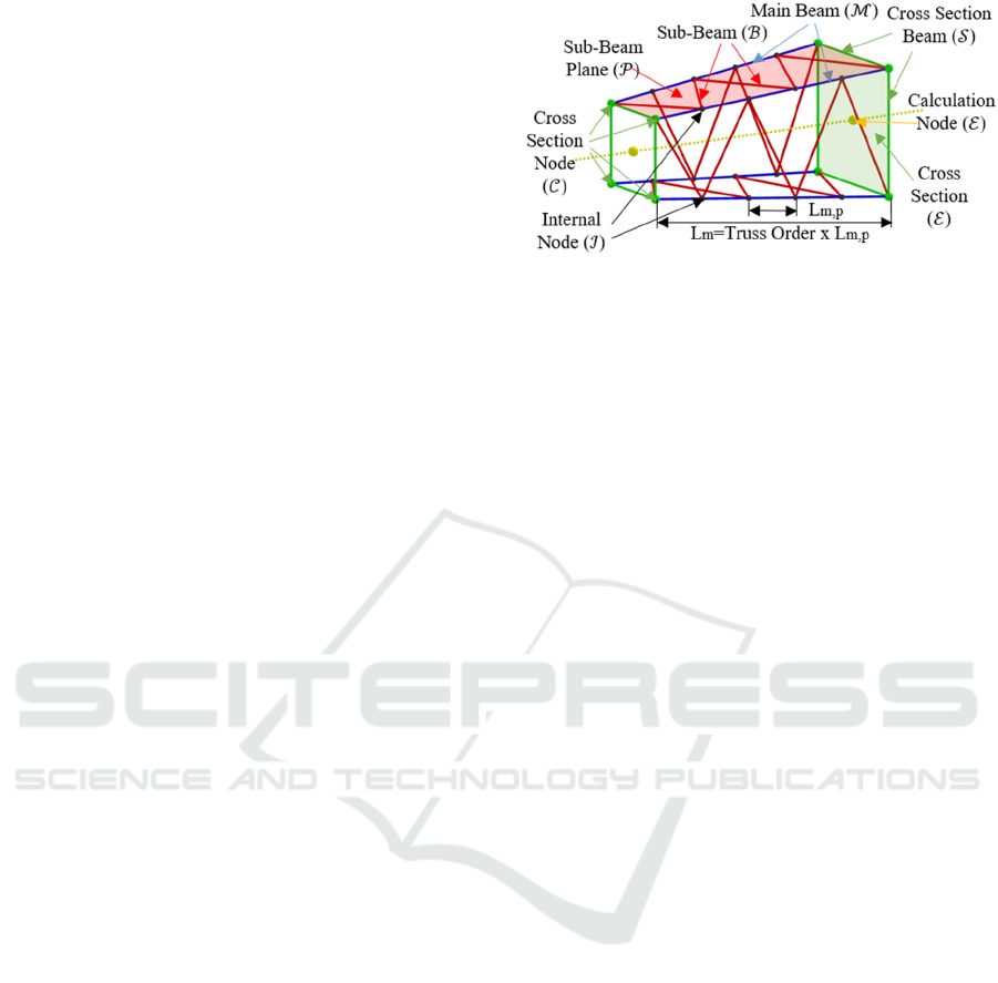
Truss Elements and Truss Order. In this paper, the
truss is defined by nodes (cross section nodes, internal
nodes), planes (cross section, sub-beam planes) and
beam elements (cross section beams, main beams,
sub-beams).
The configuration of the sub-beams is defined by
the connection form and the truss order. The sub-
beam connection form refers to the position of the
internal nodes connected by the sub-beam. Truss
order refers to the ratio of the total length of the main
beam to the minimum element length divided by the
sub-beams.
Figure 1: Definition of truss elements and truss order.
Parameters of Cross Section Nodes. According to
the rigid end section assumption, we only need to
define the position vector from the section node to
any point on the end section in this section coordinate.
Moreover, the posture of the section node can be
expressed by the angle of the end section.
Parameters of Cross Section Beams. The cross
section beams of a certain cross section 𝑠 can be
defined by the cross-section nodes.
According to the definition of beam element
above, it is required that the x-axis of the beam must
be parallel to the line connecting the two ends of the
beam when there is no deformation.
The generalized coordinates of the section node
can be expressed by the generalized coordinates of
the end section
𝒏
=Δ𝒓
‖
Δ𝒓
‖⁄
Δ𝒓
=𝒓
−𝒓
(26
)
in which s∈𝒮, k,l∈𝒞.
In addition, we define that the z-axis of cross
section beam is perpendicular to the cross section,
that is, the same as the x-axis of the cross-section
coordinate.
𝒏
=𝒏
(27
)
in which i∈ℰ.
Therefore, the rotation matrix of the nodes at both
ends of the end beam can be defined as
𝑹
=
𝒏
𝒏
𝒏
(28
)
According to assumption of rigid end section or
rigid connection, the relative rotation angle between
the coordinate system of the nodes at both ends of the
cross-section beam and the coordinate system of the
end section is constant under deformation.
𝑹
𝑹
→𝝋
,
=constant
(29
)
SIMULTECH 2021 - 11th International Conference on Simulation and Modeling Methodologies, Technologies and Applications
54
Parameters of Main Beams, Sub-beam Planes and
Internal Nodes. Main beam is defined by the two
cross section nodes of different end section.
The x-axis of the main beam is along the length
of the main beam
𝒏
=Δ𝒓
‖
Δ𝒓
‖⁄
Δ𝒓
=𝒓
−𝒓
(30
)
in which m∈ℳ
The sub-beams must be located on the surface
formed by the two main beams. We only discuss the
situation where two main beams form a plane, which
is basically the same in practical applications. The
direction of the sub-beam plane and the z-axis of the
main beam in this sub-beam plane is defined by its
normal vector.
𝒌
=𝒏
×𝒏
𝒏
,
=𝒏
,
=𝒌
(31
)
in which n∈ℳ, g∈𝒫.
The main beams belonging to different sub-beam
planes will have different directions defined in each
sub-beam plane.According to the rigid connection
assumption, the relative rotation angle between the
end node of the main beam and the cross-section node
is constant.
𝝋
,
=𝝋
,
𝑹
𝑹
,
(32
)
With the assumption of geometric continuity of
the main beam, the direction of the internal nodes on
the main beam is the same as the direction of the main
beam when it is not deformed.
Parameters of Sub-beams. The sub-beam is defined
by the main beam and the location of end nodes on
the main beam.
The x-axis of the sub-beam is defined as the unit
vector from the internal node on main beam 1 point
to the internal node on main beam 2.
𝒏
=Δ𝒓
Δ𝒓
Δ𝒓
=𝒓
,
−𝒓
,
(33
)
in which h∈ℬ, p,q∈ℐ.
The z-axis of the sub-beam is defined as the
normal direction of the sub-beam plane.
𝒏
=𝒌
(34
)
According to the rigid connection assumption, the
relative rotation angle between the end point
coordinate of the sub-beam and the corresponding
main beam coordinate is constant and must be along
the normal direction of the sub-beam plane.
𝑹
𝑹
→𝝋
,
=𝜑
,
𝒌
(35
)
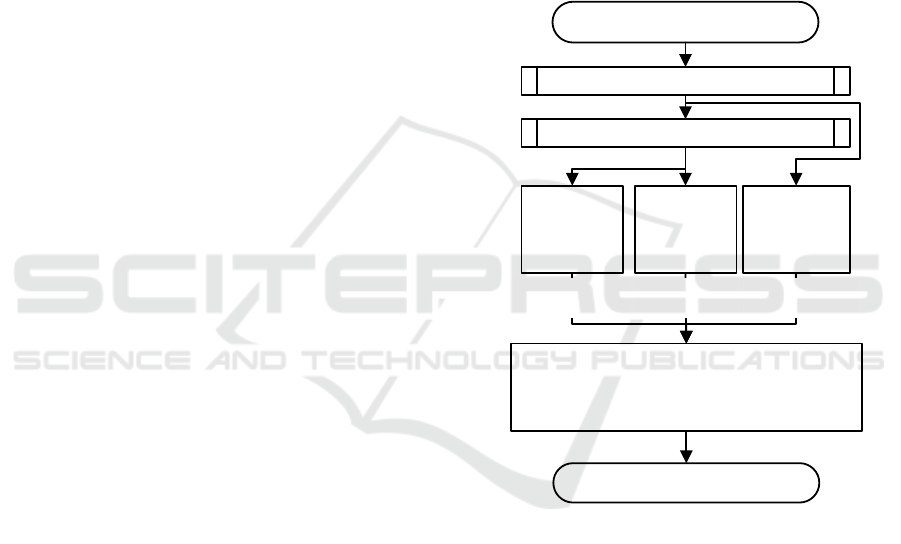
2.2.3 Calculation
The dynamics calculation of the super truss element
is composed of the following modules: cross section
node, internal node, cross section beam, main beam
and sub-beam.
Figure 2: Flow chart of dynamic calculation of super truss
element.
From the dynamic calculation flow chart, it can be
found that the calculations of the cross-section beam,
the main beam and the sub-beams do not affect each
other. Parallel calculation can effectively reduce the
single-step calculation time of the super truss
element.
Cross Section Nodes. According to the assumption
of rigid end section, the position of the cross-section
nodes can be calculated. Moreover, the posture of the
section nodes can be expressed by the angle of the end
section. Therefore, the generalized coordinates of the
section node can be expressed by the generalized
coordinates of the end section
Calculate cross section node coordinate
Mass = MainBeamMass + CrossSectionMass
+ SubBeamMass
Force = MainBeamForce + CrossSectionForce
+ SubBeamForce
Start
Super Truss Element Mass&Force
Calculate Internal Node coordinate
Calculate
Main Beam
Mass&Force
Calculate
Sub-Beam
Mass&Force
Calculate
Cross Section
Beam
Mass&Force
q
e
,dq
e
Cross Section Nodes
CrossSectionMass,
CrossSectionForce
MainBeamMass,
Main BeamFo rce
SubBeamMass,
SubBeamForce
Internal Nodes
Mass,Force
End
Super Truss Element Mass&Force
Dynamics Modelling and Simulation of Super Truss Element based on Non-linear Beam Element
55

𝒒
=
𝒓
𝝋
=
𝒓
+𝑹
𝒓
,
𝝋
𝑹
=𝑹
(
𝝋
)
(36
)
The generalized velocity and acceleration of the
cross-section node can be expressed as
d𝒒
=
𝒓
𝝎
=𝑻
d𝒒
d𝒒
=𝑻
d𝒒
+𝑻
d𝒒
(37
)
in which
𝑻
=𝑻
𝑻
𝑻
=𝑻
𝑻
where
𝑻
=
𝑰−𝑹
𝒓
,
𝟎𝑰
𝑻
=
𝟎−𝑹
𝝎
𝒓
,
𝟎𝟎
and 𝑻
is the selection matrix of the end section.
𝑻
=
𝑰𝟎
,i=1
𝟎𝑰
,i=2
Internal Nodes. Here the main deformation of the
main beam is considered to be caused by bending.
Thus, the deformation in axial direction is ignored
(Zhang et al. 2015). The global position vector of
centreline is obtained by employing the Hermite
interpolation. The velocity and acceleration of the
centroid can be expressed as
𝒓
=𝑻
d𝒒
𝒓
=𝑻
d𝒒
+𝑻
d𝒒
(38
)
In order to determine the angle coordinates, we
use the cardan angle to describe the angle change
relative to the end of Section 1
k
z
→
𝜃
y
→
𝜓
x
→
𝜑
p k
z
→
𝜃
y
→
𝜓
x
→
𝜑
l
So that the rotation matrix of cross section can be
formulated as
𝑹
=𝑹
𝑹
(
𝜃
)
𝑹
(
𝜓
)
𝑹
(
𝜑
)
(39
)
According to Hermite Interpolation, the unit
normal vector of the cross-section can be expressed
by
𝒏
=𝒓
‖
𝒓
‖⁄
(40
)
The unit normal vector of the cross-section can
also be expressed through the relative rotation angle
to end section 1
𝒏
=𝑹
𝑹
(
𝜃
)
𝑹
(
𝜓
)
𝒈
(41
)
Since the relative rotation angle is small,
according to the monotonicity of the sin-function near
zero position, two parameters of the cardan angle can
be obtained by the following formula
𝜓
=−sin
𝒈
𝑹
𝒏
𝜃
=sin
𝒈
𝑹
𝒏
cos 𝜓
(42
)
The torsion angle in the x direction is obtained by
linear interpolation
𝜑
=𝜉𝜑
𝜑
=𝜉𝜑
(43
)
The torsion angle from end section 1 to end
section 2 can be obtained by solving following
equation
𝑹
=𝑹
𝑹
(
𝜃
)
𝑹
(
𝜓
)
𝑹
(
𝜑
)
(44
)
The solution is
𝜑
=sin
𝒈
𝑹
𝑹
𝒈
cos 𝜓
𝜓
=−sin
𝒈
𝑹
𝑹
𝒈
𝜃
=sin
𝒈
𝑹
𝑹
𝒈
cos 𝜓
(45
)
in which 𝒈
=
100
.
Angular deformation vector related to cardan
angle can be written as
𝝋
=
𝜑
𝜓
𝜃
(46
)
According to the relationship between rotation
matrix and the Cartesian rotation vector, the
rotation vector 𝝋
of cross section can be
obtained by
𝑹
→𝝋
(47
)
SIMULTECH 2021 - 11th International Conference on Simulation and Modeling Methodologies, Technologies and Applications
56

The angular velocity and angular acceleration
of section 𝑐 can be written as
𝝎
=𝑻
d𝒒
=𝑹
𝝎
+𝑻
𝝋
𝝎
=𝑹
𝝎
−𝝎
𝑹
𝝎
+𝑻
𝝋
+𝑻
𝝋
=𝑻
d𝒒
+𝑻
d𝒒
(48
)
in which the rotation matrix and angular velocity with
subscript φ should be calculated using cardan angle
The generalized coordinate and generalized
velocity of internal node of main beam can be
obtained by
𝒒
=
𝒓
𝝋
d𝒒
=
𝒓
𝝎
=𝑻
d𝒒
d𝒒
=𝑻
d𝒒
𝐦
+𝑻
d𝒒
(49
)
where
𝑻
=
𝑻
𝑻
𝑻
=
𝑻
𝑻
According to the definition of the main beam, the
coordinate of end point of the main beam can be
represented by the end node coordinate of super truss
element.
d𝒒
=𝑻
d𝒒
d𝒒
=𝑻
d𝒒
+𝑻
d𝒒
(50
)
where
𝑻
=
𝑻
𝑻
𝑻
=
𝑻
𝑻
Therefore, the internal node coordinate can be
written by the coordinate of the super truss beam
element.
d𝒒
=𝑻
d𝒒
d𝒒
=𝑻
d𝒒
+𝑻
d𝒒
(51
)
where
𝑻
=𝑻
𝑻
𝑻
=𝑻
𝑻
+𝑻
𝑻
Cross Section Beam Elements. According to the
parameters of the definition of cross section nodes,
the coordinate of the end point of the cross-section
beam is depend only on cross section node.
𝒒
=
𝒓
𝝋
=
𝒓
𝝋
+𝑹
𝝋
,
(52
)
The generalized velocity and acceleration of the end
point of the cross-section beam can be expressed as
d𝒒
=
𝒓
,
𝝎
=𝑻
,
d𝒒
d𝒒
=𝑻
,
d𝒒
+𝑻
,
d𝒒
(53
)
where
𝑻
,
=𝑻
,
𝑻
𝑻
,
=𝑻
,
𝑻
𝑻
,
=
𝑰𝟎
𝟎𝑹
(𝝋
,
)
According to the definition of end beam, the
generalized coordinates of end beam can be expressed
as
𝒒
=
𝒒
𝒒
d𝒒
=
d𝒒
d𝒒
=𝑻
d𝒒
d𝒒
=𝑻
d𝒒
+𝑻
d𝒒
(54
)
where
𝑻
=
𝑻
,
𝑻
,
𝑻
=
𝑻
,
𝑻
,
The mass matrix and force vector of the cross-
section beam need to be calculated through the
generalized coordinates of the cross-section beam,
and then converted to the super truss element
coordinate. The virtual power of the cross-section
beam can be written as
δ𝑝
=−δd𝒒
(
𝑴
d𝒒
+𝑭
)
=−δd𝒒
(
𝑴
d𝒒
+𝑭
)
(55
)
where
𝑴
=𝑻
𝑴
𝑻
𝑭
=𝑻
𝑴
𝑻
d𝒒
+𝑭
Main Beam Elements. Considering that internal
nodes will transmit force and moment, it is necessary
to segment the main beam according to the position
of the internal nodes (sub main beam), in order to
meet the virtual power principle. The generalized
coordinate of sub main beam can be obtained directly
using the generalized coordinate of internal nodes.
Dynamics Modelling and Simulation of Super Truss Element based on Non-linear Beam Element
57
d𝒒
=𝑻
d𝒒
d𝒒
=𝑻
d𝒒
+𝑻
d𝒒
(56
)
where
𝑻
=
𝑻
𝑻
𝑻
=
𝑻
𝑻
(57)
The virtual power of sub main beam can be written as
δ𝑝
=−δd𝒒
(
𝑴
d𝒒
+𝑭
)
=−δd𝒒
(
𝑴
d𝒒
+𝑭
)
(58)
where
𝑴
=𝑻
𝑴
𝑻
𝑭
=𝑻
𝑴
𝑻
d𝒒
+𝑭
Sub-beam Elements. According to the internal
nodes connected by the sub-beam and the constant
relative rotation between the end points of the sub-
beam and the internal nodes, the generalized
coordinates of the end points of the sub-beam can be
obtained through the internal nodes.
The generalized velocity and acceleration of the
sub-beam endpoint can be expressed as
d𝒒
=𝑻
,
d𝒒
d𝒒
=𝑻
,
d𝒒
+𝑻
,
d𝒒
(59
)
where
𝑻
,
=𝑻
,
𝑻
𝑻
,
=𝑻
,
𝑻
𝑻
,
=
𝑰𝟎
𝟎𝑹
(𝝋
,
)
Therefore, the generalized coordinates of sub-
beam can be written as
d𝒒
=𝑻
d𝒒
d𝒒
=𝑻
d𝒒
+𝑻
d𝒒
(60
)
where
𝑻
=
𝑻
,
𝑻
,
𝑻
=
𝑻
,
𝑻
,
The virtual power of sub-beam can be written as
δ𝑝
=−δd𝒒
𝑴
d𝒒
+𝑭
=−δd𝒒
𝑴
d𝒒
+𝑭
(61
)
where
𝑴
=𝑻
𝑴
𝑻
𝑭
=𝑻
𝑴
𝑻
d𝒒
+𝑭
3 SIMULATION AND ANALYSIS
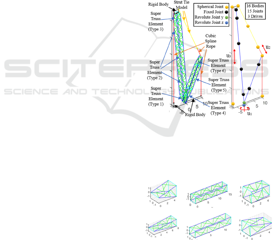
3.1 Model of a Lattice Boom System
This lattice boom system of a mobile crane consists
of a main boom, a derrick boom, strut tie rods and
ropes. The model is created using rigid-flexible
multibody dynamics method.
The configurations of body model type and joint
are shown in Figure 3.
Figure 3: Element Type (left, real model) and Joint
Configuration (right, calculation model).
The lattice boom system has now three drives: 1.
crane rotates along z-axis. 2. lift rope changes its
length. 3. angle of main boom changes.
The types of the truss elements are shown in
Figure 4.
T
yp
e 1 T
yp
e 2 T
yp
e 3
T
yp
e 4 T
yp
e 5 T
yp
e 6
Figure 4: Different Types of Super Truss Element.
SIMULTECH 2021 - 11th International Conference on Simulation and Modeling Methodologies, Technologies and Applications
58
3.2 Dynamics Tests for Truss Element
If we fix one end of the super truss element and apply
force or torque on the other end, the displacement of
the free end can reflect the stiffness of the truss beam.
Here in Figure 5 only the curves of external force or
torque and strain of Type 2 are shown as an example.
(a) Axial Stretch (b) Axial Compression
(
c
)
x-Axis Twist
(
d
)
y
-Axis Bendin
g
(
e
)
z-Axis Bendin
g
Figure 5: Strain-stress curves under different deformation
states for super truss element Type 2.
(
a
)
Axial Stretch
(
b
)
x-Axis Twist
(
c
)
y
-Axis Bendin
g
(
d
)
z-Axis Bendin
g
Figure 6: Deformation in different states for super truss
element Type 2.
It can be seen from the curve in Figure 5 that the
stresses and strains by axial force and bending are
linear.
The torsion in the x-axis will cause the strain
in the axial direction, which is caused by the main
beam rotating around the axis of super truss element
instead of its own axis.
This also makes the equivalent
torsional stiffness in x-axis of the truss not constant.
The continuous beam model cannot express this
phenomenon. The state after the deformation of the
super truss element under various conditions is shown
in Figure 6.
If we let the both end of the super truss element
free and add same force or torque on both ends. The
velocity change of the super truss element can be used
to determine the mass parameter.
From Figure 7, the angular velocity change can be
seen as linear to time. However, only the translational
velocity change in x-Axis is linear to time. In fact, due
to the discontinuity and asymmetry of the truss, it is
difficult to express the mass matrix of the truss
through a continuous beam model. Especially for
non-rectangular trusses, the determination of its
equivalent mass will become very difficult.
(
a
)
x-Axis Translation
(
b
)
x-Axis Rotation
(
c
)
y
-Axis Rotation
(
d
)
z-Axis Rotation
Figure 7: Time-Velocity curves under different force or
torque states for super truss element Type 2.
3.3 Load Lifting
(
a
)
Static State
(
b
)
Final State
Figure 8: Start State (a) and Final State (b) for lifting.
The actual motion of the crane must be relatively
smooth. In order to simulate smooth motion, we will
use the motion function in (Gao et al. 2020) to lift the
load. The start state and final state for lifting is shown
in Figure 8.
The translational displacement and velocity in z-
axis are shown in Figure 9.
Dynamics Modelling and Simulation of Super Truss Element based on Non-linear Beam Element
59
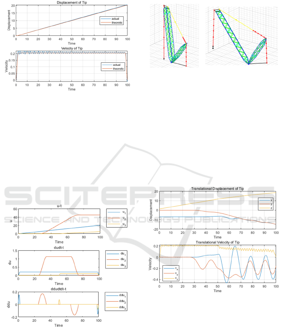
Figure 9: translational displacement and velocity in z-axis
for lifting.
3.4 Combined Motion
In practice, the motions of the mobile cranes in the
operation can be specified as three kinds, lifting,
slewing, and luffing. The slewing means the boom
system and the turntable (super-structure) rotates
along the vertical slewing axis. The luffing means to
change the distance between the payload and the
slewing axis by changing the elevation angle of the
boom. In this section, we also designed the lifting
state under the simultaneous action of multiple drives.
The combined motion can be divided into 4 stages:
Figure 10: Combined Drive Function.
1. 0 - 25s: lifting stage
2. 25 - 50s: lifting + slewing stage
3. 50 - 75s: lifting + slewing + luffing stage
4. 75 - 100s: lifting + luffing stage
(
a
)
Static State
(
b
)
Final State
Figure 11: Start State (a) and Final State (b) for combined
motion.
During the movement, the position and speed of
the load are shown in Figure 12. From the figure, we
can find that in the only lifting stage, the position of
the load changes smoothly, and the speed has only a
small vibration. The slewing of the crane has little
effect on the vertical motion of the load. The position
of the load changes smoothly in the horizontal
direction, but speed begins to fluctuate greatly. The
luffing motion of the crane has a greater influence on
the vertical direction of the lifting, the fluctuation of
the speed in the vertical direction becomes larger, and
there is a big vibration in the horizontal direction.
Figure 12: Translational Position and Velocity of the Load.
For some kinds of loads, the stability of its posture
is also very important. Therefore, in addition to the
position change of the load, we also need to consider
the angle change when it is moving. The angle change
is shown in Figure 13. We can find that in the overall
movement, the angle of the load does not change
much (the maximum angle change is less than 1
degree). Among them, the angle change caused by the
forward motion of the crane is relatively the largest,
and the angular velocity of the load vibrates violently.
SIMULTECH 2021 - 11th International Conference on Simulation and Modeling Methodologies, Technologies and Applications
60
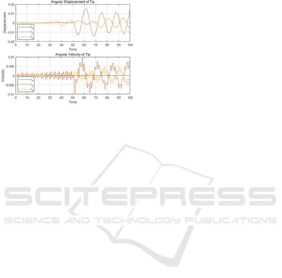
Figure 13: Posture and Angular Velocity of the Load.
4 CONCLUSION AND OUTLOOK
In order to reduce the complexity of truss beam
modelling in this paper a super truss element for
dynamic calculation is proposed. Based on three
assumptions, a parameterization method for truss
beams is established, and a dynamic calculation
method for super truss elements is proposed.
Through the stiffness experiment of super truss
elements, a reasonable method to determine the
properties of truss beams is given, and the problem of
using continuous beam elements to simulate truss
beam elements has been discovered. Finally, through
the crane movement, the feasibility of using super
truss element modelling was confirmed.
The following topics are considered as further
research:
1) Although the super truss element can greatly
reduce the number of degrees of freedom, it is still
needed to calculate each member of the truss beam in
each time step. This makes the single-step calculation
time of the ODE solver very large. Parallel computing
and other methods of accelerating computing to
reduce computing time will be studied in the future.
2) The parameterization method in this paper is
only suitable for general simple truss models. At
present, in the direction of lighter and miniaturized
machinery, more complex truss models are widely
used. These trusses may no longer meet the three
assumptions in this paper when they are deformed.
Therefore, a completer and more general truss model
is urgently needed.
ACKNOWLEDGEMENTS
The research is supported by Deutsche
Forschungsgemeinschaft (DFG) (FO 1180 1-1).
REFERENCES
Bazoune, A.; Khulief, Y. A.; Stephen, N. G. (2003): Shape
functions of three-dimensional Timoshenko beam
element. In: Journal of Sound and Vibration 259 (2), S.
473–480.
Gao, Lingchong; Zhuo, Yingpeng; Peng, Micheal
Kleeberger1 Haijun; Fottner, Johannes (2020):
Modeling and Simulation of Long Boom Manipulator
Based on Geometrically Exact Beam Theory. In:
Proceedings of the 10th International Conference on
Simulation and Modeling Methodologies, Technologies
and Applications, S. 209–216.
Günthner, W. A.; Kleeberger, M. (1997): Zum Stand der
Berechnung von Gittermast-Fahrzeugkranen. In: dhf
(03), S. 56–61.
Kammer, Daniel C.; Allen, Mathew S.; Mayes, Randy L.
(2015): Formulation of an experimental substructure
model using a Craig–Bampton based transmission
simulator. In: Journal of Sound and Vibration 359, S.
179–194.
Kleeberger, Michael (1996): Nichtlineare dynamische
Berechnung von Gittermast-Fahrzeugkranen: na.
Kleeberger, Michael; Hübner, Karl-Thomas (2006): Using
Superelements in the Calculation of Lattice-Boom
Cranes. In: Logistics Journal: referierte
Veröffentlichungen 2006 (Dezember).
Koutsovasilis, P.; Beitelschmidt, M. (2007): Model
Reduction of Large Elastic Systems: A.
Luo, Yunhua (2008): An efficient 3d timoshenko beam
element with consistent shape functions. In: Adv. Theor.
Appl. Mech 1 (3), S. 95–106.
Wang, Gang; Qi, Zhaohui; Kong, Xianchao (2015):
Geometrical nonlinear and stability analysis for slender
frame structures of crawler cranes. In: Engineering
Structures 83, S. 209–222.
Zhang, Zhigang; Qi, Zhaohui; Wu, Zhigang; Fang, Huiqing
(2015): A spatial Euler-Bernoulli beam element for
rigid-flexible coupling dynamic analysis of flexible
structures. In: Shock and Vibration 2015.
Dynamics Modelling and Simulation of Super Truss Element based on Non-linear Beam Element
61
