Motif-based Classification using Enhanced Sub-Sequence-Based
Dynamic Time Warping
Mohammed Alshehri
1,2
, Frans Coenen
1
and Keith Dures
1
1
Department of Computer Science, University of Liverpool, Liverpool, U.K.
2
Department of Computer Science, King Khalid University, Abha, Saudi Arabia
Keywords:
Time Series Analysis, Dynamic Time Warping, K-Nearest Neighbour Classification, Sub-Sequence-Based
DTW, Matrix Profile, Motifs.
Abstract:
In time series analysis, Dynamic Time Warping (DTW) coupled with k Nearest Neighbour classification,
where k = 1, is the most commonly used classification model. Even though DTW has a quadratic complexity,
it outperforms other similarity measurements in terms of accuracy, hence its popularity. This paper presents
two motif-based mechanisms directed at speeding up the DTW process in such a way that accuracy is not
adversely affected: (i) the Differential Sub-Sequence Motifs (DSSM) mechanism and (ii) the Matrix Profile
Sub-Sequence Motifs (MPSSM) mechanism. Both mechanisms are fully described and evaluated. The eval-
uation indicates that both DSSM and MPSSM can speed up the DTW process while producing a better, or at
least comparable accuracy, in 90% of cases.
1 INTRODUCTION
Today’s technology allows us to collect large amounts
of time series data. Examples include stock mar-
ket data (Ebadati and Mortazavi, 2018), weather data
(Karevan and Suykens, 2020) and electrocardiogram
data (Phinyomark and Scheme, 2018). Time series
analysis is directed at finding and extracting mean-
ingful knowledge from this data. The analysis can
take many forms, but a frequently encountered exam-
ple is time series classification where we wish to build
a model of the time series data we have and then use
this model to label a time series ú, that we have not
previously seen, according to a set of classes C.
Time series classification, whether supervised, un-
supervised or somewhere between the two, requires a
comparison of time series. The number of compar-
isons to be undertaken is the main contributing factor
to the computational complexity of time series clas-
sification. A range of techniques is available to cal-
culate similarity between two time series. Euclidean
Distance (ED) and Dynamic Time Warping (DTW)
are the most widely used techniques. Although ED
is faster, it has been shown to be less accurate than
DTW (Rakthanmanon et al., 2012; Silva et al., 2018),
and does not support comparison of time series of dif-
ferent length, whilst DTW does. On the other hand,
DTW is slower. DTW has a time complexity O(x
2
),
compared to a time complexity of O(x) for ED (where
x is the length of the time series). In the context of
supervised time series classification a range of algo-
rithms is available: Decision Trees (Brunello et al.,
2018), Artificial Neural Networks (Gamboa, 2017)
and Deep Learning (Fawaz et al., 2019). However,
k-Nearest Neighbour (kNN), with k = 1 and DTW
as the similarity measurement, remains the most fre-
quently used algorithm for time series classification
(Rakthanmanon et al., 2012; Silva et al., 2018). The
work presented in this paper is directed at reducing
the time complexity of DTW with a focus on the kNN
algorithm with k = 1.
DTW was first introduced in the speech recogni-
tion community (Sakoe and Chiba, 1978). The main
idea was to find the optimal match, the minimum
“warping distance”, wd, between two time series,
S
1
= [p
1
, p
2
,..., p
x
] and S
2
= [q
1
,q
2
,...,q
y
] (where
p
i
and q
j
are individual values in the time series, and
x and y are the time series lengths). The DTW pro-
cess can be described as follows. A distance matrix
M of size x × y is generated where the value held at
each cell m
i, j
is calculated as shown in Equation 1
(Niennattrakul and Ratanamahatana, 2009), where d
i j
is the ED between the corresponding points p
i
∈ S
1
and p
j
∈ S
2
, to which is added the minimum value
from the three “previous” cells (m
i, j
(m
i−1, j
, m
i−1, j−1
or m
i, j−1
) (Alshehri et al., 2019a). At the end of the
184
Alshehri, M., Coenen, F. and Dures, K.
Motif-based Classification using Enhanced Sub-Sequence-Based Dynamic Time Warping.
DOI: 10.5220/0010519301840191
In Proceedings of the 10th International Conference on Data Science, Technology and Applications (DATA 2021), pages 184-191
ISBN: 978-989-758-521-0
Copyright
c
 2021 by SCITEPRESS – Science and Technology Publications, Lda. All rights reserved

Table 1: Symbol Table.
Symbol Description
p or q A point in a time series described by a single value.
S A time series such that S = [p
1
, p
2
,...] (S = [q
1
,q
2
,...]), S ∈ D.
x or y The length of a given time series.
D A collection of time series {S
1
,S
2
,...,S
r
}
r The number of time series in in D.
C A set of class labels, C = {c
1
,c
2
,...}, associated with a D.
M A distance matrix measuring x × y (used for DTW)).
m
i, j
The distance value at location i, j in M.
wd A warping distance derived from M.
 The number of points in a subsequence.
w A time series subsequence {p
i
, p
i+1
,...}, such that w ∈ S
s The number of sub-sequences into which a given time series is to be split,
s = x/ (s = y/).
t The tail measured backwards from  within which a cut is to be applied to
create a sub-sequence; thus given S = [p
0
,..., p

] the cut will fall between p

and p
−t
.
W A set of s time series subsequences, {w
1
,w
2
,...w
s
} contained in a given time
series S
¯
l The number of points in a motif (used with the DSSM mechanism).
n The length of a window in a Matrix Profile (used with the MPSSM mecha-
nism).
ú A new previously unseen time series to be classifieed (labeled).
process, the minimum wd will be held at m
x,y
. Two
time series are identical if wd equates to zero. As the
value of wd increases, the similarity reduces.
m
i, j
= d
i, j
+ min{m
i−1, j
,m
i, j−1
,m
i−1, j−1
} (1)
There has been previous work directed at reduc-
ing the complexity of DTW, typically directed at re-
ducing the size of M. One example can be found
in (Alshehri et al., 2019b) where the Sub-Sequence-
Based DTW mechanism was proposed. The main
idea here was to speed up the DTW process by split-
ting the two time series to be compared into equally-
sized sub-sequences of length . Consequently, the
size of M was reduced by a factor of . The process
of DTW was then applied in each corresponding sub-
sequence simultaneously. Finally, the values held in
m
x,y
for all sub-sequence was accumulated to give fi-
nal wd value. This mechanism produced better re-
sults compared to standard DTW, not only in terms of
run-time, but also in terms of accuracy and F1-Score.
This paper builds on this idea, but instead investigates
the potential of using only a limited number of sub-
sequences. The idea is akin to the concept of mo-
tifs proposed in (Torkamani and Lohweg, 2017). In
more detail, this paper proposes two motif-based clas-
sification mechanisms founded on the Sub-Sequence-
Based DTW idea: (i) the Differential Sub-Sequence
Motifs (DSSM) mechanism and (ii) the Matrix Pro-
file Sub-Sequence Motifs (MPSSM) mechanism. The
distinction is how the motifs are identified. Using the
DSSM mechanism the set of classes, C, is used to se-
lect motifs that are good differentiators of class. Us-
ing the MPSSM mechanism, the matrix profile idea,
proposed on (Yeh et al., 2016) is used.
The remainder of this paper is organised as fol-
lows. A review of related work is presented in Section
2. The proposed DSSM and MPSSM mechanisms are
presented in Section 3. The theoretical computational
complexity of the proposed mechanisms is presented
in Section 4. The evaluation of the proposed tech-
niques is then presented in Section 5, together with a
discussion of the results obtained. The paper is con-
cluded in Section 7. For convenience, a symbol table
is given in Table 1 listing the symbols used through-
out the paper.
2 BACKGROUND AND
PREVIOUS WORK
The Sub-Sequence-Based DTW idea, first proposed
in (Alshehri et al., 2019b), was directed at speed-
ing up the DTW process by segmenting two time se-
ries S
1
and S
2
into sub-sequences. Thus, given two
time series S
1
and S
2
, these would be divided into s
sub-sequences so that we have S
1
= [U
1
1
,U
1
2
,...U
1
s
]
and S
1
= [U
2
1
,U
2
2
,...U
2
s
]. DTW was then applied to
Motif-based Classification using Enhanced Sub-Sequence-Based Dynamic Time Warping
185

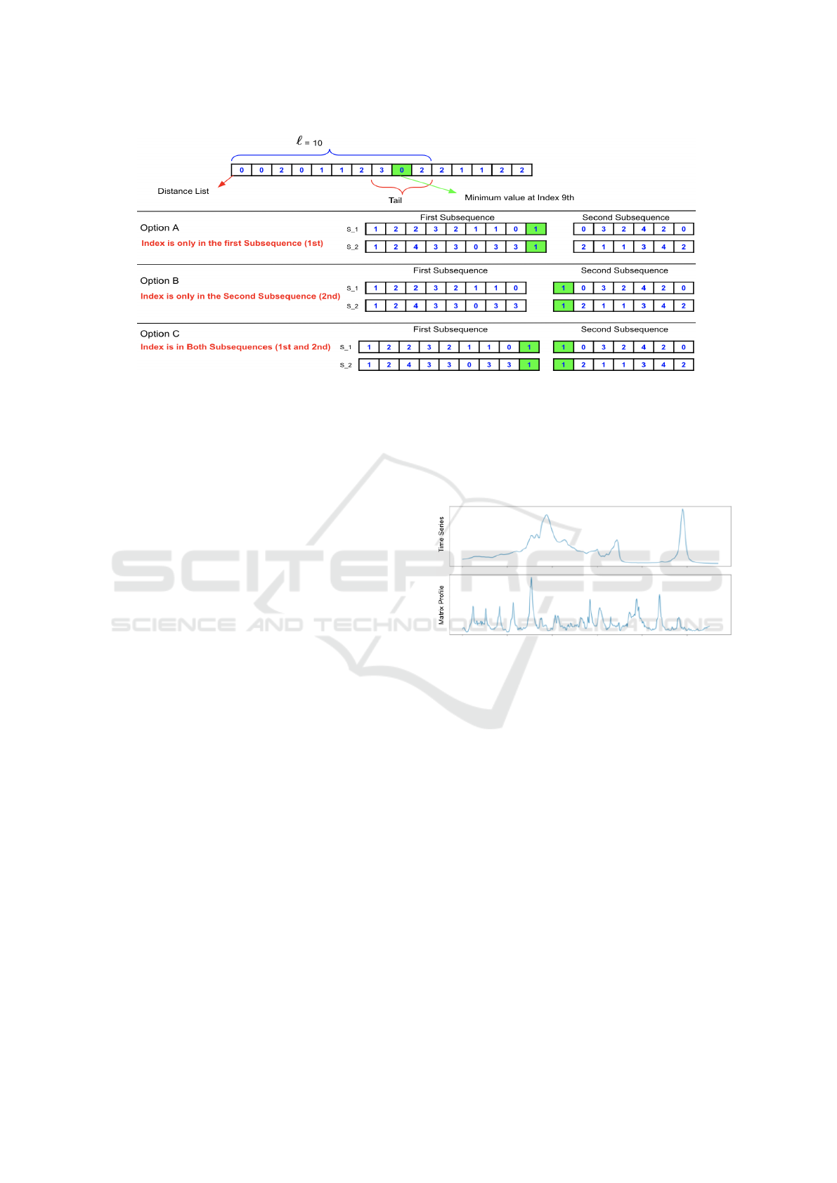
Figure 1: Segmentation examples given two time series S
1
and S
2
, and SPAO options A, B or C (Alshehri et al., 2019a).
each sub-sequence paring U
1
i
,U
2
j
where i = j. The
minimum wd values arrived at were then accumu-
lated to give a final wd value. The approach worked
well in some cases, and not so well in other cases;
this was found to be because of the use of a fixed
value for s which suited some applications, but not
all. Therefore, an improved approach, Enhanced Sub-
Sequence-Based DTW, was proposed in (Alshehri
et al., 2019a) which featured a more flexible way of
dividing a time series into sub-sequence by finding the
most appropriate size for s by using two parameters:
the maximum length of a sub-sequences  and a tail
t, measured backwards from , within which the cut
was to be applied (Alshehri et al., 2019a). Thus, given
a time series U = [p
0
,..., p

,...], the first “cut” will
fall between p

and p
−t
; and so on for further cuts.
In addition, a Split Point Allocation Option (SPAO)
was considered. This featured three alternative ways
of including the split point, identified as A, B and C, as
illustrated in Figure 1. Option A was found to provide
the best performance and was therefore used with re-
spect to the evaluation presented later in this paper.
The MPSSM mechanisms presented later in this
paper is founded on the concept of matrix profiles, as
first introduced in (Yeh et al., 2016), for finding mo-
tifs within time series. Motifs are repeating patterns
in a time series. The Matrix Profile technique has two
main components: (i) a distance profile and (ii) a pro-
file index. The distance profile is constructed using
a sliding window technique and holds “distance” val-
ues. The profile index holds indexes to sub-sequences
referenced in the distance profile. The similarity is
measured using Euclidean Distance. Only one param-
eter is used, the sliding window size n. The distance
profile is used to identify frequently occurring dis-
tances which are referenced to the index profile which
in turn references individual sub-sequences in the in-
put which are then identified as motifs. The distance
profile idea is central to the MPSSM mechanism de-
scribed later in this paper. Figure 2 gives an example
of the matrix profile generated from an original time
series.
Figure 2: Matrix Profile generation. Top: the original time
series. Bottom: the resulting Matrix Profile.
3 PROPOSED TECHNIQUES
In this section, the two proposed time series classi-
fication mechanisms, the Differential Sub-Sequence
Motifs (DSSM) mechanism and the Matrix Profile
Sub-Sequence Motifs (MPSSM), are presented. Re-
call that the objective is to speed up the DTW process
by reshaping time series to a form based on the con-
cept of motifs. Then, Enhanced Sub-Sequence-Based
DTW is applied to the reshaped time series data. The
DSSM mechanism is presented in Sub-section 3.1 and
the MPSSM mechanism in Sub-section 3.2 respec-
tively.
3.1 Differential Sub-Sequence Motifs
This sub-section presents the proposed DSSM mech-
anism. The pseudo code for the DSSM mechanism
DATA 2021 - 10th International Conference on Data Science, Technology and Applications
186

Algorithm 1: Differential Sub-Sequence Motifs.
1: input D, |C|,
¯
l
2: D
0
= {hS
0
1
,c
i
i,hS
0
2
,c
2
i,...hS
0
r
,c
r
i}, S
i
=
/
0  D
Reshaped
3: A = Temporary set of sets length |C| to hold sets
of time series
4: for ∀hS
j
,c
j
i ∈ D do  Populate A
5: A
i
= A
i
∪ hS
j
,c
j
i (i = j)
6: end for
7: for ∀A
i
∈ A do  Populate B
8: B = Temporary array [dist
1
,dist
2
,...,dist
r
],
dist
i
= 0
9: for S
j
∈ A
i
, j = 0 to j = r − 1 do
10: for ∀p
x
∈ S
j
and ∀q
x
∈ S
j+1
do
11: dist
x
∈ B = dist
x
+ abs(p
x
− q
x
)
12: end for
13: end for
14: W = [w
1
,w
2
,...,w
s
], array of sub-sequences
in B, each of length
¯
l
15: I = [i
1
,i
2
,...,i
s
], array of indexes to S
1
∈ A
i
(one-to-one match
with W )
16: E = Temporary array [dist
1
,dist
2
,...,dist
s
]
17: for ∀w
j
∈ W do  Populate E
18: dist
j
∈ E =
∑
i=
¯
l
i=0
p
i
∈ w
j
19: end for
20: F = Temporary array [count
1
,count
2
,...]
holding frequency counts
for each dist
j
∈ E
21: S
0
i
∈ D
0
= sub-sequence in S
1
∈ A
i
associated
with w
i
that has the
highest frequency count in F
22: end for
23: return D
0
is given in Algorithm 1. The inputs (line 1) are: (i)
the data set D = {hS
1
,c
i
i,hS
2
,c
2
i,...hS
r
,c
r
i}, where
each S
i
is a time series and c
i
is the associated class
label taken from the set of classes C (c
i
∈ C), (ii)
the number of classes in C and (iii) a sub-sequence
length
¯
l. The first step (line 2) is to declare the re-
shaped data set D
0
which is to be populated as the
process progresses. Next (lines 3 to 6) the time series
in D are grouped according to their associated class
and placed in a set of sets A = {A
1
,A − 2, . . . A
|C|
},
where set A
i
holds the collection of time series asso-
ciated with class c
i
. This set of sets is then processed,
lines 7 to 22, so that a reshaped input set is produced
(stored in D
0
). For each set A
i
∈ A, associated with
a particular class c
i
, a temporary array B of length r
is generated (lines 8 to 13), which holds the accumu-
lated distances for each value in the time series in A
i
.
Thus the accumulated distances between the time se-
ries for time point 1, time point 2, and so on up to time
point r (the assumption is that the input time series are
all of the same length). The array B is then, line 14,
divided into a set of non-overlapping sub-sequences,
W = {w
1
,w
2
,...,w
s
}, each of length
¯
l. An array of
indexes is also created (line 15) that links the start
of each sub-sequence in W back to the correspond-
ing sub-sequence in time series S
1
∈ A
i
; the signifi-
cance is that one of these sub-sequences will be se-
lected as the motif to represent class c
i
. A temporary
array E is then created, lines 16 to 18, to hold the ac-
cumulated distances (sum of distances) held in each
sub-sequence w
j
∈ W . Note that there is a one-to-one
correspondence between W and E. A third temporary
array F is then created (line 20) to hold the frequency
count of each distance dist
i
∈ E; the length of F will
depend on the number of unique distances held in E.
The sub-sequence in S
1
∈ A
i
which is associated with
the distance w
j
∈ W that has the highest frequency
count as listed in F, is then selected as the motif for
class c
i
to be included in D
0
(line 21); this is facilitated
by the array of indexes I created earlier (line 15). At
the end of the process D
0
will be populated with a set
of sub-sequences, representative of the input time se-
ries, one sequence per class.
Effective Sub-Sequence DTW, described earlier,
will then be used to label previously unseen time se-
ries using kNN with k = 1. Given a new time se-
ries to be labeled, ú, this is first segmented into a se-
quences of sub-sequences, each of length
¯
l. The sub-
sequences in ú will then be compared to the motifs
in D
0
and the class associated with the most similar
motif in D
0
adopted as the label for ú.
3.2 Matrix Profile Sub-Sequence Motifs
The second motif-based mechanism considered in
this paper is the MPSSM mechanism. This uses the
matrix profile technique from (Yeh et al., 2016) as
outlined in Section 2; although unlike the technique
described in (Yeh et al., 2016) an index profile is not
used. Instead the the distance profile is used as the re-
shape input data D
0
. The pseudo code for the MPSSM
mechanism is given in Algorithm 2. The input (line 1)
is the data set D = {hS
1
,c
i
i,hS
2
,c
2
i,...hS
r
,c
r
i} and
a window size n. The first step (lines 2), as in the
case of the DSSM mechanism, is to declare the re-
shaped data set D
0
which is to be populated as the
process progresses. This next step, lines 3 to 10, is
to reshaped the input D into a distance matrix which
will be stored in D
0
. Each time series S
i
∈ D is seg-
mented (line 4) into x − n + 1 sub-sequences each of
length n (recall that x is the length of the time series in
D). We then (line 5) create a comparator time series
Motif-based Classification using Enhanced Sub-Sequence-Based Dynamic Time Warping
187

T comprised of the first n points in S. Then (lines 6 to
8), for each sub-sequence w
j
∈ W we determine the
Euclidean Distance between w
j
and T and add this to
S
0
i
∈ D
0
. At the end of the process we have a distance
profile held in D
0
.
Algorithm 2: Matrix Profile Sub-Sequence Motifs.
1: input D, n
2: D
0
= {hS
0
1
,c
i
i,hS
0
2
,c
2
i,...hS
0
r
,c
r
i}, S
i
=
/
0  D
Reshaped
3: for ∀S
i
= [p
1
, p
2
,..., p
x
] ∈ D do  Create
distance profile
4: W = a list of time series sub-sequence, of
length x − n + 1, generated by moving
a window, of length n along S
i
5: T = [p
1
,..., p
n
]
6: for ∀w
j
∈ W do
7: d = distance between T and w
j
8: S
0
i
= S
0
i
∪ d
9: end for
10: end for
11: return D
0
Given a previously unseen time series, ú, this will
be compared with the contents of D
0
using Effective
Sub-Sequence-Based DTW. To do this it has to be
reshaped in the same manner as the “training” data
to give ú
0
. This is done by repeating lines 4 to 9 of
the pseudo code given in Algorithm 2, but with S
i
re-
placed with ú, and S − i
0
replaced with ú
0
.
4 TIME COMPLEXITY
The time complexity of the two proposed mechanisms
are presented in this section. When comparing two
time series S
1
and S
2
, using standard DTW, the time
complexity (DTW
compStand
) depends on the size of the
distance matrix M. The time complex is thus given by
O(x × y) where x and y are the lengths of S
1
and S
2
respectively (Alshehri et al., 2019a). If both S
1
and S
2
are of the same length (number of points in each time
series), the time complexity can be simplified to:
DTW
compStand
= O

x
2

(2)
With respect to Sub-Sequence-Based DTW (Alshehri
et al., 2019a) as first proposed in (Alshehri et al.,
2019b), the DTW time complexity, DTW
compSubS
, re-
duces to:
DTW
compSubS
= O

x
2
x ÷ 

(3)
The time complexity using the DSSM mechanism
for comparing two time series, DTW
compDSSM
, where
one time seres has been reduced to a single motif of
length , and the other has been segmented into s sub-
sequences of length , is then given by:
DTW
compDSSM
= O


2
× s

(4)
With respect to MPSSM mechanism, where we
are comparing a reshaped time series (a row in a dis-
tance profile) with another reshaped time series, each
of length x − n + 1. the time complexity will be:
DTW
compMPSSM
= O ((x − n + 1) × (x − n + 1)) (5)
where: n is the window size and x is the length of a
time series (assuming all time series are of the same
length.
When using k-nearest neighbour (kNN) classifica-
tion with k = 1, the most frequently used time series
classification model (Bagnall et al., 2017; Silva et al.,
2018), a new time series ú to be classified will need
to be compared to all records r ∈ D. The complex-
ity when using standard DTW or sub-sequence DTW
will be:
O(r × complexity × |ú|) (6)
where: (i) r is the number of records in the
kNN “bank”, (ii) complexity is either DTW
compStand
,
DTW
compSubS
or DTW
compMPSSM
, and (iii) |ú| is the
number of previously unseen time series to be labeled.
Using the DSSM mechanism, where we have only
one motif per class in the kNN bank, this reduces to:
O(|C| × DTW
compDSSM
× |ú|) (7)
5 EVALUATION
The evaluation of the proposed DSSM and MPSSM
mechanism is presented in this section. Their op-
eration was compared with: (i) Standard DTW (the
Benchmark) and (ii) Enhanced Sub-Sequence-Based
DTW with  = 40 and t = 2 and Option A as rec-
ommended in (Alshehri et al., 2019a) (see Section 2
for detail). The evaluation was conducted using kNN
with k = 1. Ten datasets taken from the UEA and
UCR Time Series repository (Bagnall et al., 2017)
were used for the evaluation reported here. Datasets
of different size of data were considered, ranging
from x = 150 to x = 2000 (time series length) and
from r = 60 to r = 781 (number of records). A
overview of the data sets used is given in Table 2. In
the table the datasets are listed according to x (Col-
umn 3). Column 5, shows the number of classes (|C|).
The evaluation objectives were:
DATA 2021 - 10th International Conference on Data Science, Technology and Applications
188

1. Parameter Settings: To identify the best param-
eters settings for the two proposed mechnisms.
2. Runtime: To compare the operation of the pro-
posed mechanisms, in terms of run time, with the
operation of Standard DTW and Effective Sub-
Sequence-Based DTW.
3. Accuracy: To compare the operation of the pro-
posed mechanisms, in terms of accuracy, with the
operation of Standard DTW and Effective Sub-
Sequence-Based DTW.
Each is discussed in turn in the following three sub-
sections, Sub-section 6 to Sub-section 6.2. For the
experiments, a desktop computer with a 3.5 GHz Intel
Core i7 processor and 28 GB, 2400 MHz, DDR3 of
primary memory was used.
6 PARAMETER SETTINGS
The results from experiments to identify best param-
eter settings for DSSM and MPSSM are given in Ta-
bles 3 and 4 respectively. Recall that the distinction
between the two is that DSSM uses a parameter
¯
l (the
number of points in a motif) while MPSSM uses a
parameter n (window size). The final column in each
table (Column 6) gives the relative run time (seconds).
The results are averages obtained using cross valida-
tion. The range of test values used for  and t were the
same as those used in (Alshehri et al., 2019a). For the
parameter
¯
l, this was defined in terms of a percentage
of the overall length of a time series, from 5% to 95%
incrementing in steps of 5%, {5%,10%,...,95%}.
Table 2: Evaluation Time Series Datasets.
ID Dataset Len. Num. Num.
No. Name (x) recs. (r) Classes
1. GunPoint 150 200 2
2. OliveOil 570 60 4
3. Trace 275 200 4
4. ToeSegment2 343 166 2
5. Car 577 120 4
6. Lightning2 637 121 2
7. ShapeletSim 500 200 2
8. DiatomSizeRed 345 322 4
9. Adiac 176 781 37
10. HouseTwenty 2000 159 2
6.1 Run Time Performance
In this sub-section, the runtime performance for the
two proposed mechanisms is considered. Table 5
gives the runtime results four the four mechanisms
considered. The runtimes for DSMM and MPSSM,
Table 3: DSSM Best Parameters, , t and
¯
l.
ID Dataset Parameters R’time
No. Name  t
¯
l (sec)
1. GunPoint 10 1 35% 3.00
2. OliveOil 40 2 90% 2.30
3. Trace 70 1 80% 6.50
4. ToeSegment2 100 1 80% 7.90
5. Car 60 2 35% 2.85
6. Lightning2 40 2 60% 5.70
7. ShapeletSim 90 2 95% 20.60
8. DiatomSizeRed 20 2 20% 6.00
9. Adiac 10 2 95% 120
10. HouseTwenty 300 5 45% 45.00
Table 4: MPSSM Best Parameters, , t and n.
ID Dataset Parameters Runtime
No. Name  t n (sec)
1. GunPoint 40 2 30 5.18
2. OliveOil 80 2 20 2.30
3. Trace 50 2 40 6.51
4. ToeSegment2 50 2 15 9.05
5. Car 50 6 35 9.10
6. Lightning2 110 2 45 9.60
7. ShapeletSim 70 2 5 20.50
8. DiatomSizeRed 20 2 40 25.11
9. Adiac 10 5 70 115
10. HouseTwenty 400 2 20 130
the last two columns, are taken from Tables 3 and 4 re-
spectively. From the table, it can be seen that the run-
time of the two proposed techniques is faster in nine
of the ten cases; with DSMM providing the best per-
formance. The exception was the Adiac data set; the
reason for this may have something to do with this be-
ing the largest data set in terms of number of records.
With respect to the DiatomSizeReduction and House-
Twenty; the runtime using DSSM was more than 10
times fastere when compared to the standard DTW.
Figure 3 shows the same runtime results as given in
Table 5, but in graph from with the datasets arranged
along the x-axis the tun time on the y-axis.
6.2 Accuracy of Performance
In this sub-section, the performance of the two pro-
posed mechanism is considered in terms of accuracy
and F1 score. The results are given in Table 6; stan-
dard deviation values are given in parenthesis. The
values given in the table are the average of Ten Cross
Validations (TCVs). Best results are highlighted in
bold font. From the Table, it can be seen that with
respect to DSSM the accuracy improved, over stan-
dard DTW and Enhanced Sub-sequence based DTW,
in five cases, and remained the same in a further three
cases. Only in two cases, ShapeletSim and Adiac,
did DSSM produce a worse performance. With re-
Motif-based Classification using Enhanced Sub-Sequence-Based Dynamic Time Warping
189

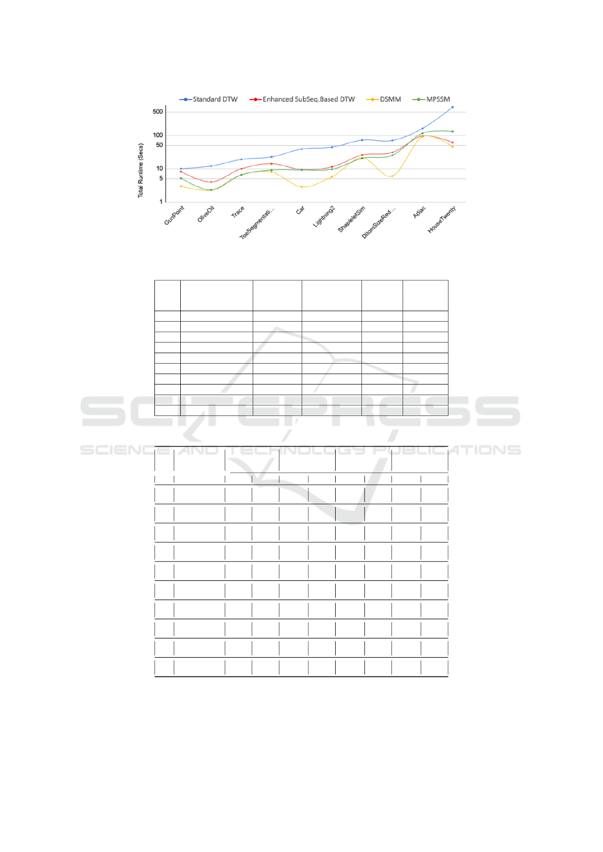
Figure 3: Total TCV runtime results (seconds) to classify each datasets.
Table 5: Total Runtime Results (seconds) using Ten Cross Validation, best results in bold font.
Standard Enhanced
ID Data Set DTW Sub-Seq. DSMM MPSSM
No. (B’mark) Based DTW
1. GunPoint 10.00 8.16 3.00 5.18
2. OliveOil 12.02 4.00 2.30 2.30
3. Trace 18.98 9.96 6.50 6.51
4. ToeSegment2 22.49 14.05 7.90 9.05
5. Car 38.69 9.45 2.85 9.10
6. Lightning2 43.90 11.33 5.70 9.60
7. ShapeletSim 71.69 25.65 20.60 20.50
8. DiatomSizeRed 69.88 30.66 6.00 25.11
9. Adiac 160.11 94.94 120.00 115.00
10. HouseTwenty 696.88 60.89 45.00 130
Table 6: Best accuracy and F1 results, overall best accuracy and F1 values highlighted in bold font.
Bencmark
Standard
DTW
Enhanced
Sub-Sequenc
Based DTW
DSSM MPSSM
ID
#
Data
set Acc F1 Acc F1 Acc F1 Acc F1
1 GunPoint
93.97
(0.04)
0.94
(0.05)
99.00
(0.02)
0.99
(0.02)
99.50
(0.01)
0.99
(0.01)
98.00
(0.02)
0.98
(0.02)
2 OilveOil
89.52
(0.15)
0.88
(0.16)
90.00
(0.10)
0.89
(0.12)
90.00
(0.10)
0.89
(0.12)
90.00
(0.08)
0.89
(0.10)
3 Trace
99.00
(0.03)
0.99
(0.03)
96.50
(0.04)
0.97
(0.04)
99.00
(0.02)
0.99
(0.02)
100.00
(0.00)
1.00
(0.00)
4
Toe
Segmentation2
89.07
(0.09)
0.88
(0.10)
92.26
(0.03)
0.92
(0.04)
95.11
(0.05)
0.95
(0.03)
88.53
(0.05)
0.88
(0.07)
5 Car
80.83
(0.07)
0.80
(0.09)
82.50
(0.10)
0.81
(0.11)
86.67
(0.11)
0.86
(0.12)
83.33
(0.09)
0.82
(0.10)
6 Lightin2
87.74
(0.09)
0.87
(0.08)
87.40
(0.08)
0.87
(0.09)
89.26
(0.06)
0.89
(0.07)
75.26
(0.13)
0.75
(0.13)
7
DiatomSize
Reduction
99.36
(0.01)
0.99
(0.01)
100.00
(0.00)
1.00
(0.00)
100.00
(0.00)
1.00
(0.00)
100.00
(0.00)
1.00
(0.00)
8 ShapeletSim
82.37
(0.09)
0.81
(0.11)
93.00
(0.04)
0.93
(0.04)
89.00
(0.05)
0.89
(0.06)
99.50
(0.01)
0.99
(0.01)
9 Adiac
64.63
(0.03)
0.62
(0.04)
64.98
(0.03)
0.62
(0.04)
64.63
(0.03)
0.62
(0.04)
53.78
(0.05)
0.52
(0.06)
10 HouseTwenty
93.75
(0.04)
0.94
(0.04)
91.17
(0.07)
0.91
(0.07)
96.25
(0.05)
0.96
(0.05)
94.29
(0.06)
0.94
(0.06)
spect to MPSSM the accuracy improved, over stan-
dard DTW and Enhanced Sub-sequence based DTW,
in five cases, and remained the same in a further
two cases. Only in three cases, ToeSegmnetation2,
Lightin2 and Adiac, did MPSSM produce a worse
performance. Again, both DSSM and MPSSM did
DATA 2021 - 10th International Conference on Data Science, Technology and Applications
190

not work well with respect to the Asiac data set (possi-
bly because of its size in terms of number of records).
In general, the proposed DSSM and MPSSM mecha-
nisms, performed better or as well as Standard DTW
or Enhanced Sub-sequence based DTW, but with an
improved run time (much improved in some cases).
From the results presented in Table 6 an argument can
be made that DSSM produced the best results.
7 CONCLUSION
In this paper, two DTW mechanisms have been pro-
posed founded on the concept of motifs: (i) the
Differential Sub-Sequence Motifs (DSSM) mecha-
nism and (ii) the Matrix Profile Sub-Sequence Motifs
(MPSSM) mechanism. Both were directed at speed-
ing up the DTW process without adversely affecting
accuracy. The operation of the proposed mechanisms
was compared with Standard DTW and Enhanced
Sub-sequence based DTW, using a kNN classification
model with k = 1 and ten time series data sets of a va-
riety of sizes; taken from the UEA and UCR (Univer-
sity of East Anglia and University of California River-
side) Time Series Classification Repository (Bagnall
et al., 2017). The evaluation demonstrated that the
proposed mechanisms outperformed the comparator
mechanisms in nine out of ten cases with respect to
run time without adversely affecting classification ac-
curacy. Out of the two proposed mechanisms DSSM
gave the best performance.
REFERENCES
Alshehri, M., Coenen, F., and Dures, K. (2019a). Effec-
tive sub-sequence-based dynamic time warping. In In-
ternational Conference on Innovative Techniques and
Applications of Artificial Intelligence, pages 293–305.
Springer.
Alshehri, M., Coenen, F., and Dures, K. (2019b). Sub-
sequence-based dynamic time warping. In KDIR,
pages 274–281.
Bagnall, A., Lines, J., Bostrom, A., Large, J., and Keogh,
E. (2017). The great time series classification bake
off: a review and experimental evaluation of recent
algorithmic advances. Data Mining and Knowledge
Discovery, 31(3):606–660.
Brunello, A., Marzano, E., Montanari, A., and Sciavicco,
G. (2018). A novel decision tree approach for the
handling of time series. In International Conference
on Mining Intelligence and Knowledge Exploration,
pages 351–368. Springer.
Ebadati, O. and Mortazavi, M. (2018). An efficient hybrid
machine learning method for time series stock market
forecasting. Neural Network World, 28(1):41–55.
Fawaz, H. I., Forestier, G., Weber, J., Idoumghar, L., and
Muller, P.-A. (2019). Deep learning for time series
classification: a review. Data Mining and Knowledge
Discovery, 33(4):917–963.
Gamboa, J. C. B. (2017). Deep learning for time-series
analysis. arXiv preprint arXiv:1701.01887.
Karevan, Z. and Suykens, J. A. (2020). Transductive lstm
for time-series prediction: An application to weather
forecasting. Neural Networks, 125:1–9.
Niennattrakul, V. and Ratanamahatana, C. A. (2009).
Learning dtw global constraint for time series classifi-
cation. arXiv preprint arXiv:0903.0041.
Phinyomark, A. and Scheme, E. (2018). An investigation
of temporally inspired time domain features for elec-
tromyographic pattern recognition. In 2018 40th An-
nual International Conference of the IEEE Engineer-
ing in Medicine and Biology Society (EMBC), pages
5236–5240. IEEE.
Rakthanmanon, T., Campana, B., Mueen, A., Batista, G.,
Westover, B., Zhu, Q., Zakaria, J., and Keogh, E.
(2012). Searching and mining trillions of time se-
ries subsequences under dynamic time warping. In
Proceedings of the 18th ACM SIGKDD international
conference on Knowledge discovery and data mining,
pages 262–270. ACM.
Sakoe, H. and Chiba, S. (1978). Dynamic programming
algorithm optimization for spoken word recognition.
IEEE transactions on acoustics, speech, and signal
processing, 26(1):43–49.
Silva, D. F., Giusti, R., Keogh, E., and Batista, G. E. (2018).
Speeding up similarity search under dynamic time
warping by pruning unpromising alignments. Data
Mining and Knowledge Discovery, pages 1–29.
Torkamani, S. and Lohweg, V. (2017). Survey on time se-
ries motif discovery. Wiley Interdisciplinary Reviews:
Data Mining and Knowledge Discovery, 7(2):e1199.
Yeh, C.-C. M., Zhu, Y., Ulanova, L., Begum, N., Ding,
Y., Dau, H. A., Silva, D. F., Mueen, A., and Keogh,
E. (2016). Matrix profile i: all pairs similarity joins
for time series: a unifying view that includes mo-
tifs, discords and shapelets. In 2016 IEEE 16th in-
ternational conference on data mining (ICDM), pages
1317–1322. Ieee.
Motif-based Classification using Enhanced Sub-Sequence-Based Dynamic Time Warping
191