
Comparing Classifiers’ Performance under Differential Privacy
Milan Lopuhaä-Zwakenberg, Mina Alishahi, Jeroen Kivits, Jordi Klarenbeek,
Gert-Jan van der Velde and Nicola Zannone
Department of Mathematics and Computer Science, Eindhoven University of Technology, Eindhoven, The Netherlands
Keywords:
Differential Privacy, Classifier Construction, Accuracy Comparison.
Abstract:
The application of differential privacy in privacy-preserving data analysis has gained momentum in recent years.
In particular, it provides an effective solution for the construction of privacy-preserving classifiers, in which
one party owns the data and another party is interested in obtaining a classifier model from this data. While
several approaches have been proposed in the literature to employ differential privacy for the construction of
classifiers, an understanding of the difference in performance of these classifiers is currently missing. This
knowledge enables the data owner and the analyst to select the most appropriate classification algorithm and
training parameters in order to guarantee high privacy requirements while minimizing the loss of accuracy.
In this study, we investigate the impact of the use of differential privacy on three well-known classifiers, i.e.,
Naïve Bayes, SVM, and Decision Tree classifiers. To this end, we show how these classifiers can be trained in a
differential privacy setting and perform extensive experiments to evaluate the effect of this privacy enforcement
on their performance.
1 INTRODUCTION
In the data-driven society of the 21st century, machine
learning algorithms are largely employed to infer addi-
tional knowledge and intelligence from the increasing
amounts of data available in the Internet (Marr, 2019).
In particular, classifiers have been widely used in
many real-world applications, such as face and speech
recognition, text analysis, fraud and anomaly detection,
recommendation system, weather forecasting, medical
image analysis, and biometric identification. A clas-
sifier assigns labels (classes) to new instances based
on its model trained on data whose classes are known
beforehand.
Classifiers are often trained under the assumption
that the underlying data is freely accessible. How-
ever, this assumption may not hold when training data
contains sensitive information as its publication might
raise the data owners’ privacy concerns. Consider, for
instance, a situation in which a hospital owns a dataset
describing patient information, including age, address,
gender, symptoms, and diseases. A classifier trained
on this dataset might leak sensitive information about
the individual patients.
To address this issue, a large body of work has
been devoted to train a classifier on datasets containing
sensitive information in such a way that the privacy of
the individuals whose data is present in the dataset is
guaranteed. Existing privacy-preserving solutions can
be categorized into two main classes. One class com-
prises cryptographic-based approaches that securely
train a classifier over protected data (Khodaparast et al.,
2019). These approaches, however, are not scalable
both in terms of execution runtime and bandwidth
usage (Naehrig et al., 2011). The other class com-
prises solutions relying on data anonymization tech-
niques, in which the data under analysis is perturbed
before being released, e.g.,
k
-anonymity,
`
-diversity,
and
t
-closeness (Sheikhalishahi et al., 2021). These
anonymization techniques have been criticized for not
being rigorous enough in protecting the individuals’
confidential information, and differential privacy is
emerging as the de-facto privacy standard for data
anonymization (Dwork et al., 2006). It addresses the
weaknesses of other anonymization techniques by lim-
iting the disclosure of private information of individual
records when published data aggregates information
in the dataset.
The rigorous privacy guarantees offered by differ-
ential privacy has led to its broad application in the
field of privacy-preserving data analysis. In particular,
differential privacy is used to introduce noise during the
training of classification algorithms, where the noise is
scaled according to the sensitivity of the training algo-
rithm. One of the main scenarios in which differential
privacy is applied is the training of classifiers, where
50
Lopuhaä-Zwakenberg, M., Alishahi, M., Kivits, J., Klarenbeek, J., van der Velde, G. and Zannone, N.
Comparing Classifiers’ Performance under Differential Privacy.
DOI: 10.5220/0010519000500061
In Proceedings of the 18th International Conference on Security and Cryptography (SECRYPT 2021), pages 50-61
ISBN: 978-989-758-524-1
Copyright
c
2021 by SCITEPRESS – Science and Technology Publications, Lda. All rights reserved
one party owns the data (containing sensitive informa-
tion) and the other party is interested in obtaining a
classifier trained over that data.
In this setting, multiple classification algorithms
have been extended to incorporate differential privacy,
e.g., Nearest Neighbor (Gursoy et al., 2017), Naïve
Bayes (Vaidya et al., 2013), Support Vector Machine
(SVM) (Chaudhuri et al., 2011), and Decision Tree
(Jagannathan et al., 2009). However, there is still a lack
of understanding on the impact of differential privacy
on their classification accuracy. Such knowledge would
enable the data owner and the analyst (model requester)
to decide which classifier to be trained according to (i)
dataset properties, such as dataset size, (ii) structural
properties of the classification algorithm, and (iii) the
amount of privacy required (
ε
in differential privacy).
Accordingly, this study aims to answer the following
research questions:
RQ1.
Which dataset properties influence the accuracy
of differentially private classifiers?
RQ2.
How does the accuracy of different classifica-
tion algorithms change when applied in a differential
privacy setting?
RQ3.
How is classifier accuracy affected by the pri-
vacy level enforced?
To answer these questions, we investigate three
well-known classification algorithms, namely the Naïve
Bayes, SVM and Decision Tree classifiers in a differen-
tial privacy setting. We show how these classification
algorithms can be adapted to train differentially pri-
vate classifiers and apply them to several largely-used
benchmark datasets. For each classification algorithm,
we analyze the effect of dataset properties and pri-
vacy levels on the classifier accuracy. The experiment
results show that in a differential privacy setting, no
classification algorithm is a one-size-fits-all solution
for all datasets and privacy levels. Nonetheless, under
some conditions one might outperform the others. For
example, our experiments show that a differentially
private SVM classifier returns higher accuracy when
the training dataset is large; on the other hand, the ac-
curacy of a Decision Tree classifier mainly depends on
the privacy level where the accuracy notably increases
when the privacy level is relaxed.
The contribution of this work can be summarized
as follows:
•
We show how three well-known classification al-
gorithms can be adapted to the differential private
setting and prove that these adaptations satisfy the
prescribed privacy level.
•
We apply the revised algorithms to several bench-
mark datasets and empirically evaluate classifier
accuracy with respect to the dataset properties and
privacy level.
training
data
training
process
classifier
model
predicted
label
unlabeled
data
free access
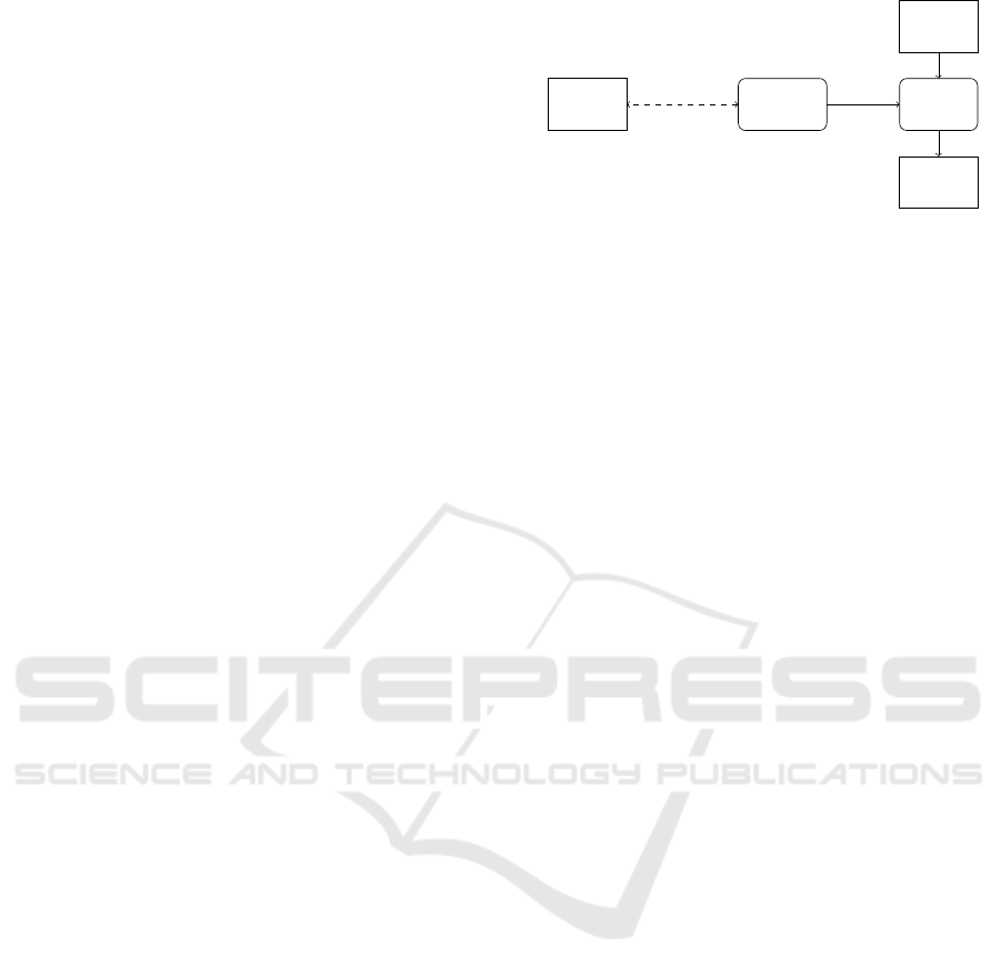
Figure 1: Classifier learning setting.
•
Based on the experiment results, we draw recommen-
dations to guide data owners and analysts in the selec-
tion of a classification algorithm for training a classi-
fier and directions for future work to improve the state-
of-the-art in differentially private classifier learning.
Outline. The remainder of the paper is organized as
follows. The next section presents the classification
algorithms studied in this work. Section 3 presents
the differential privacy classifier learning setting and
discusses the differentially private counterparts of the
classification algorithms. Sections 4 and 5 describe our
experimental setup and results, respectively. Section 6
discusses related work, and Section 7 concludes the
paper and provides directions for future work.
2 CLASSIFICATION
ALGORITHMS
In this work, we consider a classifier learning setting in
which an analyst aims to train a classifier based on the
data owned by another party. The setting is depicted
in Figure 1. We assume the training data consists of a
dataset
D
with
n
rows
~x
, which is described by a set of
attributes
A
and a distinct class attribute
C
(hereafter
we assume that
C
is a categorical attribute). Each row
~x
is a vector in which each element
x
A
is a value of
attribute
A ∈ A
and a class
x
C
. We write
¯x
for the
unlabeled row, i.e., for
~x
with the class
x
C
removed.
The analyst’s goal is to create a classifier, which can
be used to predict the class
x
0
C
of a new unlabeled
observation
¯x
0
. The analyst has free access to
D
, which
is used to train the classifier. When the classifier is
trained, it is published to the general public to be used
in the classification of new unlabeled data.
Next, we describe the three classification algorithms
studied in this work.
2.1 Naïve Bayes Classifier
Naïve Bayes classifier is a probabilistic classifier built
based on Bayes’ theorem and assumes the attributes
describing the data to be mutually independent. For-
Comparing Classifiers’ Performance under Differential Privacy
51

mally, for an unlabeled data point
¯x
, the conditional
probability of
¯x
being class
c
is denoted by
p(c|¯x)
and
(with the use of Bayes theorem) is computed as:
p(c|¯x) =
p(c)p( ¯x|c)
p( ¯x)
=
p(c)
∏
A∈A
p(x
A
|c)
p( ¯x)
(1)
where
p(c)
is the probability of class
c
to occur in
the dataset,
p( ¯x|c)
is the conditional probability that
¯x
occurs given it is labeled
c
, and
p( ¯x)
is the probability
of
¯x
to occur.
1
These probabilities are computed by
observing frequencies in the dataset. The classifier
assigns a class label
ˆc
to given data with a maximum a
posteriori probability as follows:
ˆc = argmax
c
p(c)
∏
A∈A
p(x
A
|c) (2)
This equation is equivalent to Eq. 1, removing the
constant value
p( ¯x)
in the denominator. From this
formula, it can be inferred that for constructing a Naïve
Bayes classifier, it is enough to compute the conditional
probabilities and the probability of each class label.
For a class
c
, a categorical attribute
A
, and a value
v ∈ A
, the conditional probability
p(x
A
= v|c)
and the
probability p(c) are computed as:
p(x
A
= v|c) =
n
Avc
n
c
, p(c) =
n
c
n
, (3)
where
n
Avc
is the number of rows
~x
in
D
with
x
A
= v
and
x
C
= c
and
n
c
is the number of rows with
x
C
= c
.
For a numerical attribute
A
and
z ∈ R
, the distribution
of
x
A
given
x
C
= c
is assumed to be normal, and its
probability density function is computed as:
p(x
A
= z|c) =
1
√
2πσ
Ac
e
(z−µ
Ac
)
2
2σ
2
Ac
, (4)
where
µ
Ac
is the mean value of
x
A
among the rows
~x
of
D
with class
c
, and
σ
Ac
is the standard deviation of
these values.
2.2 Support Vector Machine
The Support Vector Machine (SVM) algorithm is a clas-
sifier defined based on a statistical learning framework,
in which the class attribute is binary, i.e., the classes are
±1
, and each attribute
A
is numerical. As such we can
represent each
¯x
as a point in
|A|
-dimensional space.
The aim of the SVM training algorithm is to find a
hyperplane in this space that best separates the sets of
points corresponding to the two labels. The degree to
1
The second equivalence of (1) is derived by assuming
that attributes are independent.
which a hyperplane, represented by a normal vector
¯w
,
fails at separating the sets of points is measured by
J( ¯w,D) =
1
n
n
∑
i=1
l
h
(x
i
C
( ¯w · ¯x
i
)) +
Λ
2
|| ¯w||
2
, (5)
where
x
i
C
∈ {±1}
is the class of the
i
-th data point,
¯w · ¯x
i
is the inner product of
¯w
with the unlabeled data
point
¯x
i
, and
l
h
is the Huber loss function given, for a
fixed parameter h > 0, by
l
h
(z) =
0 if z > 1 +h,
1
4h
(1 + h −z)
2
if |1 −z|≤ h,
1 −z if z < 1 −h.
(6)
The term
Λ
2
|| ¯w||
2
in (5) is to prevent overfitting. Fol-
lowing (Chaudhuri et al., 2011), we take
h = 0.05
and
Λ = 10
−2.5
. The SVM returns the
¯w
that minimizes
(5), i.e., ˆw = argmin
¯w
J( ¯w,D).
2.3 Decision Tree Classifier
A Decision Tree classifier is a classifier that takes the
form of a rooted tree, which is iteratively trained from
the top (root) to down (leaves). Each leaf is labeled
with a class and each internal node corresponds to an
attribute in which the outgoing edges are the attribute-
values. A new data point is classified by starting from
the root and passing along its attribute-values until it
reaches a leaf. The class label of the associated leaf is
returned as the class label of the new instance.
Among the existing Decision Tree classifiers,
we consider the Classification And Regression Tree
(CART) algorithm (Breiman et al., 1984) for its sim-
ple training process. CART is a binary decision tree,
where each attribute
A ∈ A
only takes values
{0,1}
and the class attribute
C
can take more than two values.
The tree is built recursively from the root. At every
node the attribute that gives the best splitup is selected.
Formally, it is defined as follows.
The purity of node
N
(i.e., its homogeneity in
terms of class labels) is measured with the Gini index,
denoted by G(N ), and it is computed as:
G(N ) = 1 −
∑
c∈C
p
N
(x
C
= c)
2
, (7)
where
p
N
is the probability among all dataset rows
that end up in node
N
when walking from the
root. Note that
G(N ) = 0
iff all rows in
D
N
have
the same class. The CART classifier selects the
attribute whose split creates the children with the
least average Gini index (the purest children), i.e.,
SECRYPT 2021 - 18th International Conference on Security and Cryptography
52

A
best
= argmin
A∈A
∑
v∈{0,1}
p
N
(x
A
= v)G(N
A,v
), (8)
where
N
A,v
is the child of
N
with value
v
in the splitup
along with
A
. More concretely, for a given
A
and
v ∈ {0, 1}
and class
c
, and for a fixed
N
, let
m
Avc
be
the number of rows
~x
in
D
that end up at node
N
and that satisfy
x
A
= v
,
x
C
= c
. The best attribute is
selected as:
A
best
= argmin
A∈A
∑
v∈{0,1}
(
∑
c
m
Avc
)
2
−
∑
c
m
2
Avc
(
∑
c
m
Avc
)
∑
v
0
,c
m
Av
0
c
. (9)
If the stopping condition is reached, then
N
is a leaf,
and we assign to
N
the class that is most prevalent
among the training items that end up in
N
, i.e.,
ˆc =
argmax
c
m
c
,
, where
m
c
is the number of rows
~x
in
D
that end up at node N and that satisfy x
C
= c.
While theoretically one can continue splitting up
nodes until all attributes have appeared in the tree
structure, this generally results in overfitting. Therefore,
the algorithm is stopped when a maximum depth
d
is reached. We take
d = d
√
me
, which satisfies the
best trade-off between the underfitting and overfitting
of the Decision Tree model (for the selected dataset)
(Mantovani et al., 2018).
3 DIFFERENTIAL PRIVACY
CLASSIFIER LEARNING
To measure information leakage when classifiers are
trained over sensitive data, we use the de facto standard
metric named Differential Privacy (DP) defined as
follows (Dwork et al., 2006).
Definition 3.1.
Two datasets are called adjacent if
they differ in at most one row. Let
ε ∈ R
≥0
, and let
f
be an algorithm operating on datasets. We say that
f
satisfies
ε
-Differential Privacy if for all adjacent
datasets D,D
0
and all sets of possible outputs S:
P( f (D) ∈ S) ≤ e
ε
P( f (D
0
) ∈ S). (10)
By ensuring that the probability distributions on the
output space originating from two input datasets cannot
differ too much,
ε
-DP provides plausible deniability
about any row’s true value, even if all other rows are
compromised. The lower
ε
, the stronger privacy
ε
-DP
guarantees. To ensure privacy in the classifier learning
setting, we demand that a classifier training algorithm
satisfies
ε
-DP. Thus, we aim to solve the following
problem:
Problem 1.
Given a privacy level
ε
and a dataset
D
,
determine the
ε
-DP classifier training algorithm
Q
that maximizes the accuracy of the classifier Q (D).
Many classifiers are trained by retrieving infor-
mation from the dataset through numerical queries.
In this case, one can ensure
ε
-DP by making sure
the responses to queries satisfy differential privacy.
DP on a single query can be incorporated as follows.
Let
ϕ
be a numerical function on datasets, and let
s := max |ϕ(D)−ϕ(D
0
)|
, where the maximum is taken
over all adjacent
D,D
0
. Suppose a query asks for
ϕ(D)
.
Then the response
L(ϕ,ε) = ϕ(D) + Lap(0,s/ε), (11)
where
Lap(0,s/ε)
is a Laplace random variable with
mean
0
and scale parameter
s/ε
, is
ε
-DP. Occasionally
we will need responses that are positive, in which case
we will use
L
+
(ϕ,ε) = max{L(ϕ, ε),α}
, where
α
is
a small positive number that should be substantially
smaller than
ϕ(D)
. Since most of our queries are counts
and therefore integers, we use
α = 10
−5
throughout.
The response
L
+
(ϕ,ε)
is
ε
-DP as well. The following
Theorem, which follows from standard properties of
differential privacy (Dwork et al., 2006; Nguyen et al.,
2013), shows that such DP responses can be used to
construct DP classifier training algorithms:
Theorem 3.1.
Let
Q
be a classifier training algorithm,
accessing the database via queries. Suppose that each
row of the dataset is accessed through at most
m
queries
and that the response to each query is
ε
m
-DP. Then,
Q
is ε-DP.
3.1 ε-DP Naïve Bayes Classifier
To train the Naïve Bayes classifier in the
ε
-DP setting,
we mainly follow the work presented in (Vaidya et al.,
2013) with few adjustments. Specifically, 1) we have
modified the definition of standard deviation sensitivity
coming from using a different definition of adjacent
datasets, and 2) we consider the effect of multiple
queries by applying the lower value of
ε
per query
(Theorem 3.1) such that the final algorithm satisfies
ε
-DP. Algorithm 1 details the process including our
contribution and it can be summarized as follows.
Naïve Bayes relies on the dataset via the queries
n
Avc
,
n
c
,
µ
Ac
and
σ
Ac
for all
A
c
∈ A
(cf. Section 2.1).
To insert differential privacy, we instead use the noisy
versions of these values as:
L
+
(n
Avc
,ε
0
),L
+
(n
c
,ε
0
),L
+
(σ
Ac
,ε
0
),L(µ
Ac
,ε
0
), (12)
where
ε
0
is chosen such that the collection of noisy
answers as a whole satisfies ε-DP. More concretely,
ε
0
=
ε
1 + #{categorical A}+ 2#{numerical A}
. (13)
Comparing Classifiers’ Performance under Differential Privacy
53

Algorithm 1: Construction of
ε
-DP Naïve Bayes
classifier.
Data: Privacy parameter ε.
Result: Prior probabilities p(c); Conditional
probabilities p(x
A
= v|c) for each class,
categorical attribute, and value of that
attribute; Obfuscated mean ˜µ
Ac
and
standard deviation
˜
σ
Ac
for each class and
numerical attribute.
1 ε
0
←
ε
1+#{categorical A}+2#{numerical A}
;
2 for each class c do
3 ˜n
c
← L
+
(n
c
,ε
0
);
4 p(c) ←
˜n
c
n
;
5 for each categorical A, each value v ∈ A do
6 ˜n
Avc
← L
+
(n
Avc
,ε
0
);
7 p(x
A
= v|c) =
˜n
Avc
˜n
c
;
8 end
9 for each numerical A do
10 ˜µ
Ac
← L(µ
Ac
,ε
0
);
11
˜
σ
Ac
← L
+
(σ
Ac
,ε
0
);
12 end
13 end
Note that in (12) we use
L
+
for the counts and the stan-
dard deviation because they are assumed to be positive,
and L for the mean because it has no such restriction.
To calculate the expressions in relations (12), we
need to know their sensitivities. The sensitivities of the
counts
n
Avc
and
n
c
satisfy
s = 1
. We assume that for
each numerical attribute
A
, a lower bound
l
A
and upper
bound
u
A
are public knowledge. Then, the sensitivity
of µ
Ac
and σ
Ac
, respectively, are given as
s
µ
Ac
=
u
A
−l
A
n
c
, s
σ
Ac
=
u
A
−l
A
√
n
c
. (14)
Theorem 3.2. Algorithm 1 satisfies ε-DP.
Proof.
Every row in dataset is queried in one
n
c
, in
one
n
A
v
c
for each categorical attribute
A
, and in one
µ
Ac
and one
σ
Ac
for each numerical attribute
A
, so the
total amount of times each row is queried is
1 + #{categorical A}+ 2#{numerical A}. (15)
The result now follows from Theorem 3.1.
Compared to (Vaidya et al., 2013), we work with
ε
0
rather than
ε
, we have a different formula for
s
σ
A
c
in (14),
and we use
L
+
to round up certain negative responses,
rather than resampling until a positive response appears.
These changes are necessary to ensure ε-DP.
Algorithm 2: Construction of
ε
-DP SVM classi-
fier.
Data: Privacy parameter ε; Huber parameter h;
overfitting parameter Λ.
Result: Separating hyperplane ¯w
priv
.
1 ε
0
← ε −log
1 +
1
nhΛ
+
1
4n
2
h
2
Λ
2
;
2 if ε
0
> 0 then
3 ε
00
← ε
0
;
4 Λ
0
← Λ;
5 else
6 ε
00
←
ε
2
;
7 Λ
0
←
1
2nh(e
ε/4
−1)
;
8 end
9 draw
¯
b according to p(
¯
b = ¯z) ∝ e
−
ε
00
2
||¯z||
;
10 ¯w
priv
← argmax
¯w
1
n
∑
n
i=1
l
Huber
( ¯w · ¯x
i
,x
i
C
) +
Λ
0
2
|| ¯w||
2
+
1
n
¯
b · ¯w;
3.2 ε-DP SVM Classifier
We adopt the
ε
-DP implementation of SVM introduced
in (Chaudhuri et al., 2011), which is detailed in Algo-
rithm 2 and works as follows. In SVM, the resulting
hyperplane
¯w
can leak information about
D
, since it
minimizes an objective function
J
depending on
D
.
To avoid this, the objective function is perturbed so
that it does not rely on any row in
D
significantly.
More precisely, instead of the objective function
J
from Section 5, we use
J
priv
( ¯w,D) =
1
n
n
∑
i=1
l
h
( ¯w · ¯x
i
,x
i
C
) +
Λ
0
2
|| ¯w||
2
+
1
n
¯
b · ¯w
(16)
where
¯
b
is a random vector, whose probability distribu-
tion is defined below, and
Λ
0
depends on the choice of
Λ
and the privacy parameter
ε
. More concretely, given
ε, Λ and the Huber parameter h, we define
ε
0
= ε −log
1 +
1
nhΛ
+
1
4n
2
h
2
Λ
2
, (17)
ε
00
=
ε
0
, if ε
0
> 0
ε
2
, otherwise,
(18)
Λ
0
=
(
Λ, if ε
0
> 0
1
2nh(e
ε/4
−1)
, otherwise,
(19)
and
¯
b
is drawn according to
P(
¯
b = ¯z) ∝ e
−
ε
00
2
||¯z||
. The
algorithm then outputs the hyperplane
¯w
priv
= argmin
¯w
J
priv
( ¯w,D).
Theorem 3.3
(Theorem 9 of (Chaudhuri et al., 2011))
.
Algorithm 2 satisfies ε-DP.
SECRYPT 2021 - 18th International Conference on Security and Cryptography
54

Algorithm 3: Construction of
ε
-DP Decision
Tree classifier.
Data: Privacy parameter ε; Maximum depth d.
Result: Rooted tree T with labeled edges and
leaves.
1 ε
0
←
ε
|A|(d+1)
;
2 create root R ;
3 R .expandable ← True;
4 while #{expandable nodes} > 0 do
5 choose expandable node N ;
6 if N .depth = d then
7 for each class c do
8 ˜m
c
← L(m
c
,ε
0
);
9 end
10 N .label ← argmax
c
˜m
c
;
11 else
12 for each attribute A not set on path
R → N do
13 for v, c ∈ {0,1} do
14 ˜m
vc
← L
+
(m
Avc
,ε
0
);
15 end
16 G(A) ←
∑
v
(
∑
c
˜m
vc
)
2
−
∑
c
˜m
2
vc
(
∑
c
˜m
vc
)
(
∑
v
0
,c
˜m
v
0
c
)
;
17 end
18 A ← arg min
A
G(A);
19 create nodes N
0
,N
1
;
20 add labeled edges N
A=0
−→N
0
,N
A=1
−→N
1
;
21 N
0
.expandable,N
1
.expandable ← True;
22 end
23 N .expandable ← False;
24 end
3.3 ε-DP Decision Tree Classifier
An overview of differentially private Decision Tree
classifiers is given in (Fletcher and Islam, 2019). We
follow its general framework, adapted to the CART
classifier as presented in Algorithm 3. It works by
replacing the counts
m
Avc
and
m
c
with differential
privacy equivalents. More precisely, instead of
m
c
we
use the noisy version
L(m
c
,ε
0
)
, where
ε
0
=
ε
|A|(d+1)
, in
which
d
is the depth of the tree. The Gini impurity
needs positive counts as inputs, so we use
L
+
(m
Avc
,ε
0
)
.
Both these noisy counts have sensitivity s = 1.
Theorem 3.4. Algorithm 3 satisfies ε-DP.
Proof.
At each level of the tree, each row of the training
dataset is present in at most 1 node
N
. At
N
, it is
present in exactly one of the
m
c
if
N
is a leaf, and
in exactly one
m
Avc
for each attribute
A
if
N
is an
interior node. Hence each row is queried at most
|A|(d + 1)
times, and by Theorem 3.1, Algorithm 3
satisfies ε-DP.
Table 1: Dataset statistics.
Name Type #Attributes #Instances
Adult Mix 14 48 842
Mushroom Categorical 22 8 000
Nursery Categorical 8 12 960
Congressional Voting Binary 16 435
SPECT Heart Binary 22 267
Skin Segmentation Numerical 3 245 057
4 EXPERIMENTAL ANALYSIS
The experimental analysis aims to assess and compare
the classifiers’ performance when they are trained in
an
ε
-DP setting w.r.t. dataset properties (
RQ1
), clas-
sification algorithm (
RQ2
) and privacy level (
RQ3
).
Next, we present the experimental setup, the datasets
used for the experiments and the evaluation approach.
Experiment Setup.
We implemented the classifica-
tion algorithms both in a non-private (Section 2) and
an
ε
-DP setting (Algorithms 1, 2, and 3) in Python.
2
.
The privacy levels ε used to train the classifiers in the
ε
-DP setting are taken from the set
E = {10
−11
,0.001,
0.005,0.01,0.05, 0.1,0.25, 0.5,0.75,1}.
Datasets.
For our experiments we selected six datasets
from the UCI repository
3
. Table 1 summarizes the
statistics of the selected datasets.
Adult:
4
The dataset describes 48842 individuals using
14 attributes such as age, occupation, education. The
class attribute represents their income, which has two
possible values: ‘
> 50K
’ and ‘
< 50K
’. The attributes
are both numerical and categorical.
Mushroom:
5
This dataset describes 8000 hypothetical
samples of mushrooms, characterized using 22 cate-
gorical attributes, such as cap shape. The samples are
classified into two classes: edible and poisonous.
Nursery:
6
This dataset has originally been developed
to rank applications for nursery schools. The dataset
includes 12960 instances, described with 8 categorical
features such as health situation. The records are
classified into five classes, each representing a level of
being recommended for the position.
Congressional Voting:
7
This dataset includes votes for
each of the U.S. House of Representatives Congress-
men on the 16 key votes identified by the CQA. The
dataset includes 435 records, described with binary
2
The codes of our experiments are available in
https://github.com/jeroenkivits/seminar
3https://archive.ics.uci.edu/ml/datasets/
4https://archive.ics.uci.edu/ml/datasets/adult
5https://archive.ics.uci.edu/ml/datasets/Mushroom
6https://archive.ics.uci.edu/ml/datasets/nursery
7https://archive.ics.uci.edu/ml/datasets/Congressional
+Voting+Records
Comparing Classifiers’ Performance under Differential Privacy
55

attributes, such as immigration, where the records are
labeled either democrat or republican.
SPECT Heart:
8
The dataset describes diagnosing of
cardiac Single Proton Emission Computed Tomogra-
phy (SPECT) images. Each of the patients is classified
into two categories: normal and abnormal. It contains
267 instances that are described by 23 binary attributes.
Skin Segmentation:
9
This dataset comprises 245057
samples of face images of people. Each sample is
described by its RGB value (3 numerical attributes)
and is classified into two classes: skin and non-skin.
Given that the selected SVM and Decision Tree
algorithms are respectively applicable on numerical
and binary attributes, we convert the attributes of the
selected datasets in such a way that they respect the
requirements of these algorithms. For SVM, integer
numbers are randomly assigned to the distinct values
of categorical attributes. For Decision Tree, each
attribute-value of a categorical attribute is considered
as an attribute by itself, where if a record satisfies that
attribute-value the value 1 is assigned (the value 0 is
assigned, otherwise). For continuous attributes, the
median value is used to assign 1 to attribute-values
higher than the median value and 0 otherwise.
Evaluation Approach.
We measure the classifiers’
performance in terms of their accuracy. Classifier
accuracy is assessed using 10-fold cross-validation. It
is worth noting that the accuracy of
ε
-DP classifiers
is affected by the randomness introduced both by the
partitioning of the datasets and by the
ε
-DP noise,
where the latter has an especially large effect on accu-
racy. To mitigate the effect of randomness and to get a
clear picture of the average accuracy, we have repeated
each 10-fold cross-validation for 100 runs for each
ε
value for
ε
-DP Naïve Bayes and SVM classifiers. As
ε
-DP Decision Tree classifiers showed a more stable
behaviour, we repeated the experiments 10 times for
Decision Tree. The parameters of classifiers have been
tuned to their highest performance with respect to each
selected dataset in order to allow for a fair comparison.
Criteria for RQ1: Research question RQ1 aims to
understand the effect of dataset properties on classifier
accuracy in an
ε
-DP setting. To this end, we investigate
how classifier accuracy varies for datasets with different
sizes and number of attributes.
Criteria for RQ2: To investigate the effect of built-in
properties of classifiers on their accuracy when trained
in an
ε
-DP setting, we study the performance of clas-
sification algorithms when used in an
ε
-DP setting
independently from the dataset. To this end, we com-
pute the average classifier accuracy over all datasets.
8https://archive.ics.uci.edu/ml/datasets/SPECT+Heart
9https://archive.ics.uci.edu/ml/datasets/skin+segmentation
To verify whether the accuracy difference between
classification algorithms used in an
ε
-DP setting is sta-
tistically significant, we use a non-parametric statistical
test, named the Wilcoxon test (Wilcoxon, 1945). The
Wilcoxon test can be adapted to our problem as follows.
Definition 4.1
(Wilcoxon Test)
.
Given two classifica-
tion algorithms, let
d
i
be the signed difference between
the performance scores of the classifiers obtained by
applying each algorithm on a given dataset for a given
privacy level. The differences
d
i
(
1 ≤ i ≤ N
where
N
is the number of possible combinations of datasets and
privacy levels to which the classification algorithms
are applied) are ranked based on the absolute values
(average rank is assigned for equal performances). Let
R
+
denote the sum of the ranks for datasets and privacy
level on which
d
i
> 0
, and let
R
−
be the sum of the ranks
for datasets and privacy level on which
d
i
< 0
(dividing
the sum of the ranks for which d
i
= 0 evenly), i.e.,
R
+
=
∑
d
i
>0
rank(d
i
) +
1
2
∑
d
i
=0
rank(d
i
) (20)
R
−
=
∑
d
i
<0
rank(d
i
) +
1
2
∑
d
i
=0
rank(d
i
) (21)
Let T = min(R
+
,R
−
), then
z =
T −
1
4
N(N + 1)
q
1
4
N(N + 1)(2N + 1)
(22)
is approximately distributed normally. Under this con-
dition, the difference between the accuracy distribution
of the two classification algorithms is statistically signif-
icant (i.e., the null hypothesis is rejected) if the
p
-value
is less than or equal to a given significance level σ.
In our experiments, we require a 95% confidence
interval, which corresponds to σ = 0.05.
To get insight into the performance of classification
algorithms when used in an
ε
-DP setting compared to
the non-private setting, we compute
•
Accuracy (no privacy): the classifier accuracy in the
non-private setting.
•
Average accuracy (
ε
-DP): the average accuracy of
ε-DP classifiers over all ε values.
•
Ratio: the effect size of employing
ε
-differential
privacy compared to a non-private learning setting
computed as the average accuracy of
ε
-DP classifiers
over all privacy level
ε ∈ E
divided by the classifier
accuracy obtained in a non-private setting.
Criteria for RQ3: To assess the impact of privacy
levels on classifier accuracy, we analyze, for each
ε
value in
E
, the distribution of the classifier accuracy
over all selected datasets and classification algorithms.
SECRYPT 2021 - 18th International Conference on Security and Cryptography
56
To measure the effect size of
ε
on the classifier
accuracy, we use the classifier accuracy obtained in
the non-private setting (Accuracy (no privacy)) as
the baseline and compute, for each
ε
-DP classifier,
the classifier accuracy ratio as the ratio between the
classifier accuracy in the
ε
-DP setting and the accuracy
of the corresponding baseline classifier. Intuitively,
the classifier accuracy ratio represents to what extent
enforcing a given privacy level affects classifier
accuracy compared to the non-private setting.
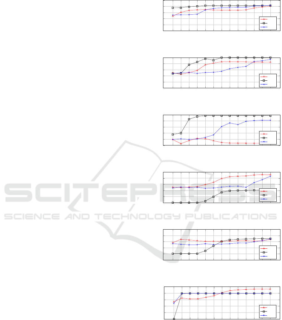
5 RESULTS
We computed the accuracy of
ε
-DP Naïve Bayes, SVM,
and Decision Tree classifiers on each selected dataset
for all privacy levels in
E
. The results of classifiers
accuracy over Adult, Mushroom, Nursery, Congres-
sional Voting, SPECT Heart, and Skin datasets, are
respectively shown in Figures 2a, 2b, 2c, 2d, 2e, and 2f.
RQ1: Which Dataset Properties Influence the Ac-
curacy of ε-DP Classifiers?
From Figure 2 we can
observe that SVM classifiers are typically accurate
when trained over datasets with a large number of
records (Adult, Mushroom, Nursery, and Skin Sep-
aration), while it returns low accuracy when trained
over small datasets (SPECT Heart and Congressional
Voting). This is due to the SVM structure in which the
hyperplane is determined based on the support vectors’
distances. When the dataset comprises a large number
of records, the noises added through differential privacy
negligibly affect the hyperplane location. On the other
hand, the accuracy of Naïve Bayes classifiers depends
neither on the number of attributes nor on the number
of records. As shown in Figure 2, for datasets with
an equal number of attributes (Mushroom and SPECT
Heart) or a large number of records (Mushroom and
Nursery), the Naïve Bayes classifier returns different
trends of accuracy. This could be because the accuracy
of Naïve Bayes classifier mainly depends on: i) the dis-
tribution of attributes’ values, and ii) the independence
of attributes (Jiang et al., 2007). Similarly, the results
show that the accuracy of Decision Tree classifiers does
not depend on the number of attributes and dataset size.
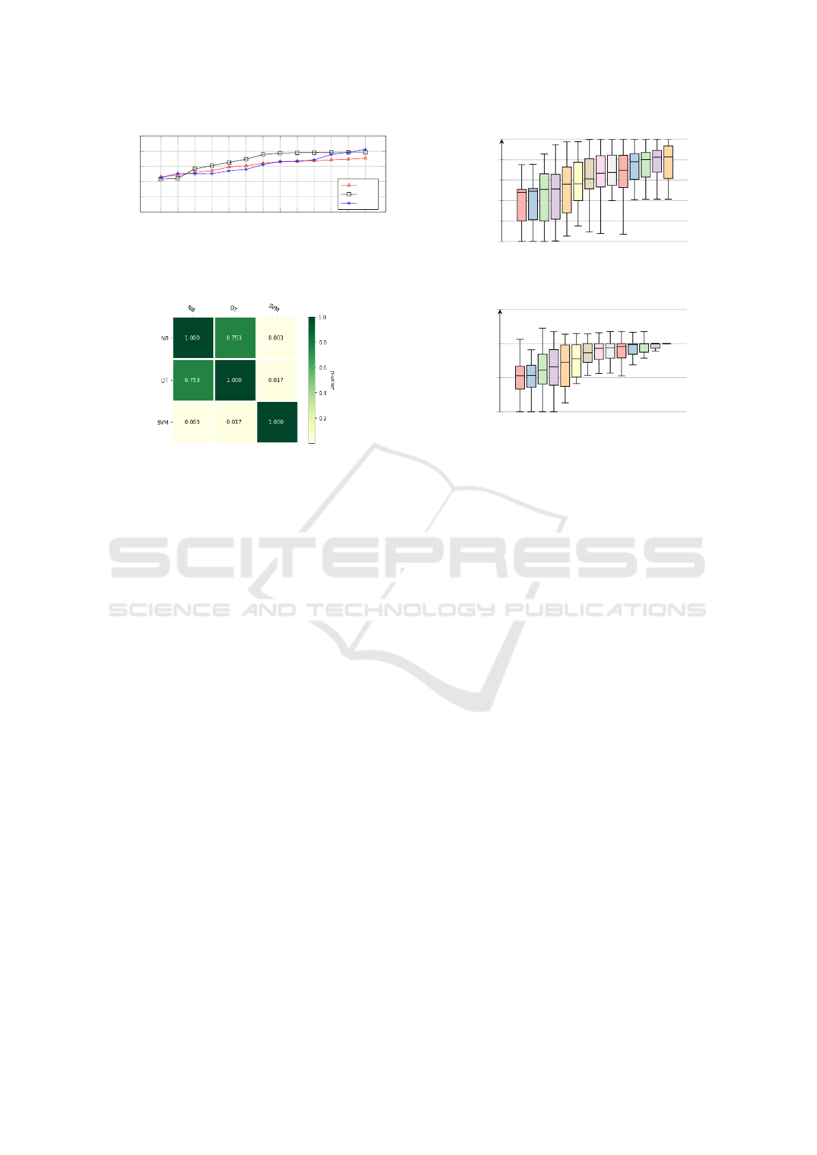
RQ2: How Does the Accuracy of Different Clas-
sification Algorithms Change when Trained in an
ε-DP Setting?
The average accuracy of the classifica-
tion algorithms when used in an
ε
-DP setting over all
datasets is reported in Figure 3. It can be observed that,
on average, SVM (for
ε
values higher than
0.005
and
lower than 3) outperforms the other two classification
algorithms. However, for small
ε
values, Naïve Bayes
and Decision Tree show slightly better performances.
10
−11
0.001
0.005
0.01
0.05
0.1
0.25
0.5
0.75
1
3
5
10
0
0.2
0.4
0.6
0.8
1
Privacy level ε
Accuracy
NB
SVM
DT
(a) Adult Dataset.
10
−11
0.001
0.005
0.01
0.05
0.1
0.25
0.5
0.75
1
3
5
10
0
0.2
0.4
0.6
0.8
1
Privacy level ε
Accuracy
NB
SVM
DT
(b) Mushroom Dataset.
10
−11
0.001
0.005
0.01
0.05
0.1
0.25
0.5
0.75
1
3
5
10
0
0.2
0.4
0.6
0.8
1
Privacy level ε
Accuracy
NB
SVM
DT
(c) Nursery Dataset.
10
−11
0.001
0.005
0.01
0.05
0.1
0.25
0.5
0.75
1
3
5
10
0
0.2
0.4
0.6
0.8
1
Privacy level ε
Accuracy
NB
SVM
DT
(d) Congressional Voting Dataset.
10
−11
0.001
0.005
0.01
0.05
0.1
0.25
0.5
0.75
1
3
5
10
0
0.2
0.4
0.6
0.8
1
Privacy level ε
Accuracy
NB
SVM
DT
(e) SPECT Heart Dataset.
10
−11
0.001
0.005
0.01
0.05
0.1
0.25
0.5
0.75
1
3
5
10
0
0.2
0.4
0.6
0.8
1
Privacy level ε
Accuracy
NB
SVM
DT
(f) Skin Separation Dataset.
Figure 2: Accuracy of Naïve Bayes, SVM, Decision Tree
classifiers trained in an
ε
-DP setting for different values of
ε
.
For low privacy levels (
ε
higher than 3), Decision Tree
returns the most accurate results. Overall, Decision
Tree classifiers show, in general, a higher improvement
Comparing Classifiers’ Performance under Differential Privacy
57
10
−11
0.001
0.005
0.01
0.05
0.1
0.25
0.5
0.75
1
3
5
10
0
0.2
0.4
0.6
0.8
1
Privacy level ε
Accuracy
NB
SVM
DT
Figure 3: Average accuracy of the classification algorithms
when used in an ε-DP setting over all datasets.
Figure 4: Heatmap of Wilcoxon test on mutual comparison
of performance between classification algorithms applied in
an ε-DP setting in terms of p-values.
when the privacy requirements are relaxed compared
to the other types of classifiers, i.e., the accuracy shows
a more noticeable increase for increasing ε values.
We used the Wilcoxon test to verify the statistical
significance of these differences. Figure 4 depicts the
heatmap of mutual comparison of
ε
-DP classifiers’
performance in terms of
p
-values. The lower
p
-value
(lighter color) shows more confidence in rejecting
the null hypothesis (i.e., more different performance).
Figure 4 shows that the null hypothesis of the Wilcoxon
test is rejected in the mutual comparison of SVM
with both Decision Tree (
p = 0.017
) and Naïve Bayes
(
p = 0.003
) classification algorithms, i.e., SVM shows
a different behaviour compared to the other algorithms.
On the other hand, the Wilcoxon test fails to reject the
null hypothesis when comparing the accuracy of Naïve
Bayes and Decision Tree, i.e., these algorithms show
similar performance.
A comparison between the accuracy achieved by the
classification algorithms when trained in a non-private
setting and in an
ε
-DP setting along with the effect size
of the accuracy difference between these settings (Ra-
tio) is reported in Table 2. The results in the non-private
setting show that for the selected datasets, on average,
the Decision Tree classification algorithm outperforms
the other two classification algorithms. However, SVM
shows better performance than the other two algorithms
when used in an
ε
-DP setting. The ratio shows that the
Naïve Bayes classification algorithm is the most stable
between the
ε
-DP and non-private settings, indicating
10
−11
0.001
0.005
0.01
0.05
0.1
0.25
0.5
0.75
1
3
5
10
no privacy
0
0.2
0.4
0.6
0.8
1
Average Accuracy
(a) Distribution of classifier accuracy for different ε
10
−11
0.001
0.005
0.01
0.05
0.1
0.25
0.5
0.75
1
3
5
10
no privacy
0
0.5
1
1.5
Accuracy Ratio
(b)
Distribution of classifier accuracy ratio for different
ε
Figure 5: Distribution of classifier accuracy and classifier
accuracy ratio for different ε values.
that it is the one less affected by the ε-DP noise.
RQ3: How Is Classifier Accuracy Affected by the
Privacy Level Enforced?
Figure 2 and Figure 3 show
that classifier accuracy decreases with the decrease of
ε
(i.e., for higher privacy requirement). SVM classifiers
perform poorly for some datasets (Nursery, Congres-
sional Voting and Skin Separation) when trained using
very small values of
ε
(Figure 2), although on average
perform only slightly worse than Decision Tree and
Naïve Bayes classifiers (Figure 3). Decision Tree clas-
sifiers show sudden increments of accuracy for some
ε
values, which can be due to the recursive structure of
this algorithm. In the construction of
ε
-DP Decision
Tree classifiers, the noise is added at every level and
each subtree can be constructed using a set of data with
a different distribution of values.
Figure 5 shows the distribution of classifier accu-
racy and classifier accuracy ratio for different
ε
values
over all classification algorithms and datasets. Each
box represents the distribution over 18 classifiers (3
classification algorithms applied to 6 datasets) for the
associated ε value.
Figure 5a shows a high variation in the accuracy of
ε
-DP classifiers (represented by the size of boxes and
length of whiskers) for every
ε
value. This variation
is especially notable for
ε
values lower than (equal to)
0.1. For
ε
values greater than 3, the distributions are
similar. This suggests the selection of a higher privacy
level in this range results in a small accuracy cost.
SECRYPT 2021 - 18th International Conference on Security and Cryptography
58

Table 2: Accuracy comparison between classification algorithms when applied in a non-private learning setting (Accuracy (no
privacy)) and in an
ε
-DP learning setting (Average accuracy (
ε
-DP)). The ratio measures the effect size of training a classifier
in an ε-DP setting compared to a non-private setting.
Classifier Measurement Adult Mushroom Nursery SPECT Congress Skin Average
NB
Accuracy (no privacy) 0.8208 0.8472 0.0834 0.5337 0.9135 0.9239 0.6871
Average accuracy (ε-DP) 0.6905 0.7458 0.1148 0.6204 0.7374 0.7763 0.6130
Ratio 0.8412 0.8803 1.3772 1.1624 0.8073 0.8922 0.9934
SVM
Accuracy (no privacy) 0.8288 0.9990 0.9747 0.6995 0.4139 0.7914 0.7846
Average accuracy (ε-DP) 0.8131 0.8892 0.8794 0.5014 0.2454 0.7918 0.6867
Ratio 0.9811 0.8901 0.9022 0.7167 0.5929 1.0001 0.8473
DT
Accuracy (no privacy) 0.8450 1.0000 0.8248 0.7388 0.9538 0.7926 0.8592
Average accuracy (ε-DP) 0.7059 0.6620 0.5427 0.5636 0.5893 0.7685 0.6387
Ratio 0.8354 0.6620 0.6580 0.7628 0.6179 0.9696 0.7510
In Figure 5b, the small boxes for
ε ≥ 0.25
, with
median values close to 1, show that classifier accuracy
is not considerably affected when the classifiers are
trained in an
ε
-DP setting for this range of
ε
(for the
selected datasets). For
0.005 ≤ ε < 0.25
, the result
shows more variation where the accuracy of
ε
-DP
classifiers can be slightly or significantly worse than
the one of classifiers trained in a non-private setting.
For
ε ≤0.001
, we can observe that the median value is
close to 0.5, indicating that, on average, the accuracy of
classifiers trained in the
ε
-DP setting halves compared
to the classifiers trained in a non-private setting.
Discussion.
In this work, we have selected three
well-known classifiers, namely Naïve Bayes, SVM,
and Decision Tree classifiers, and trained them in an
ε
-DP setting. We then explored the impact of dataset
properties, classification algorithms, and privacy levels
(in terms of differential privacy) on classifier accuracy.
Our analysis shows that none of the selected clas-
sifiers is a one-size-fits-all solution for all datasets and
privacy levels. Nonetheless, based on their inherent
structural properties, the required privacy level, and the
dataset properties, we found some interesting results
on classifiers’ performance trained in the
ε
-DP setting:
•
The ratio values reported in Table 2 show that the
Naïve Bayes classifier returns the most similar ac-
curacy between the private and non-private settings.
This specifically suggests the application of the dif-
ferentially private Naïve Bayes classifier in datasets
in which the non-private version is accurate.
•
The private SVM classifier is quite accurate when it
is trained over large datasets due to its structure.
•
The Decision Tree classifiers show increased ac-
curacy when privacy constraints are relaxed. This
could result from the fact that on the selected datasets,
the non-private Decision Tree classifiers also return
the most accurate results. Further investigation is
required to study this trend.
•
The mutual comparison of
ε
-DP classifiers’ perfor-
mance (in terms of the Wilcoxon test) shows that
probability-based classification algorithms behave
almost similarly when trained in an ε-DP setting.
•
For the selected datasets, classifier accuracy does not
change when the privacy level
ε
varies in a specific
range of values. This suggests the data owner and an-
alyst need to find the maximum privacy level for their
dataset which will not significantly affect accuracy.
It should be noted that there exist several other
alternative classification algorithms for Naïve Bayes,
SVM and Decision Tree classifiers compared to the
ones selected for this study. For instance, ID3 and
C4.5 are two types of Decision Trees, the polynomial
and RBF kernel-based SVM are other types of SVM
classifiers, and the Bernoulli and Gaussian are two
types of Naïve Bayes classifiers. Nonetheless, we
expect that the selection of an alternative classification
algorithm will not considerably affect our findings.
This claim and the other aforementioned findings of
this study needs more work to investigate the results on
a wider range of datasets, different types of classifiers,
and other classification algorithms in an ε-DP setting.
6 RELATED WORK
In recent years, privacy-preserving machine learning,
including classification, regression, clustering, and
dimensionality reduction, has received increasing at-
tention (Ji et al., 2014). This attention has resulted
in several solutions in the field of differential privacy
classification. Existing approaches in this field usually
ensure differential privacy by employing one of the
following general methods:
1.
Each row in the dataset is obfuscated, and the
training algorithm is run on the resulting data.
2.
Queries to the dataset originating from the training
algorithm are answered with a noisy result set.
3.
Once the classifier has been trained, noise is added
to its parameters before its release.
The first method, called Local Differential Privacy (Ka-
Comparing Classifiers’ Performance under Differential Privacy
59

siviswanathan et al., 2011), provides strong privacy
guarantee in training the classifiers in a differential pri-
vacy setting (Gong et al., 2020). For instance, the Naïve
Bayes classifier has been implemented with Local Dif-
ferential Privacy, i.e., with a non-interactive obfuscated
dataset (Yilmaz et al., 2019). While this method has the
advantage that it does not require a trusted data aggrega-
tor, it comes at an undesirable utility cost (Arachchige
et al., 2019). Accordingly, under the condition that
data has already been collected by a trusted aggregator,
this extra privacy guarantee is not needed.
The second method has been widely used as an ef-
fective tool in privacy-preserving classification, when
one party owns the data and another party is interested
in obtaining a classifier model on this sensitive non-
public data (Fletcher and Islam, 2019). This approach
has been used to enforce differential privacy on Naïve
Bayes classifier (Vaidya et al., 2013), which replaces the
dataset queries in the standard Naïve Bayes algorithm
with differentially private ones. This methodology has
been improved in (Zafarani and Clifton, 2020) by using
smooth sensitivity, a differential privacy technique that
lowers the amount of random noise on each query, while
retaining the same level of privacy. Differential private
SVM in a nonlinear environment has been addressed
with the use of kernel methods based on random projec-
tions (Rahimi and Recht, 2008). The accuracy of these
methods can be increased by perturbing and then solv-
ing the dual problem (Zhang et al., 2019). The methods
in (Jain and Thakurta, 2013) offer a weaker form of pri-
vacy, namely
(ε,δ)
-differential privacy, but can be ap-
plied to a wider range of kernel functions. All these ap-
proaches result in a model that does not leak unwanted
information about the training data. Depending on the
precise implementation, these approaches may have the
additional privacy guarantee that private information
is kept from the analyst as well. An overview of dif-
ferentially private Decision Tree algorithms is given in
(Fletcher and Islam, 2019). In particular, the methodol-
ogy proposed in (Blum et al., 2005) replaces the dataset
queries in a non-private Decision Tree algorithm by
differentially private equivalents. Since under differen-
tial privacy, having more queries decreases utility, one
can improve upon this by using algorithms that require
fewer dataset queries (Friedman and Schuster, 2010).
The last method adds noise to the model’s param-
eters before the model is published e.g., the optimal
hyperplane of the SVM classifier is perturbed (Chaud-
huri et al., 2011), or a random forest is created inde-
pendently of the database, and noise is then added to
the leaves’ class predictions taken from the database
(Jagannathan et al., 2009). While this approach needs
fewer queries per tree, one needs multiple trees to
get decent accuracy. In this setting, in (Jayaraman
and Evans, 2019) the evaluation of differential privacy
mechanisms for two machine learning algorithms pre-
sented to understand the impact of different choices of
ε
and different relaxations of differential privacy on
both utility and privacy. Adding noise to the classifier’s
parameters after it is trained usually results in lower
accuracy compared to previous two methods.
Our work employs the second method in which
noise is added to the analyst’s queries during the train-
ing of the classifier. Specifically, we showed how
Naïve Bayes, SVM, and Decision Tree classifiers can
be constructed in an
ε
-DP setting and compared their
performance. While some work in the literature com-
pares the impact of privacy in the context of classifier
learning, e.g., the costs of training different classifiers
using Homomorphic Encryption (Sheikhalishahi and
Zannone, 2020), to the best of our knowledge no prior
work has focused on the comparison of classifiers’
performance in a differential privacy setting.
7 CONCLUSION
This paper provides a comparison of classifiers’ per-
formance when they are trained in an
ε
-DP setting.
Three well-known classifiers, namely Naïve Bayes,
SVM and Decision Tree, have been trained under the
assumption that one party owns the data and the other
party is interested in obtaining the classifier’s model
respecting
ε
-differential privacy. Our experimental
results show that depending on dataset properties, clas-
sifier structure, and privacy level
ε
one classifier might
outperform the other ones.
In future work, we plan to extend our work to a
thorough comparison considering a wider range of
well-known classifiers (e.g.,
k
Nearest Neighbor, Ran-
dom Forest) including different types of each classifier
(e.g., different SVM algorithms) on a broader set of
benchmark datasets trained in an ε-DP setting.
ACKNOWLEDGEMENTS
This work was supported by NWO grant 628.001.026
and H2020 EU funded project SECREDAS [GA
#783119].
REFERENCES
Arachchige, P. C. M., Bertok, P., Khalil, I., Liu, D., Camtepe,
S., and Atiquzzaman, M. (2019). Local differential
privacy for deep learning. IEEE Internet of Things
Journal, 7(7):5827–5842.
SECRYPT 2021 - 18th International Conference on Security and Cryptography
60

Blum, A., Dwork, C., McSherry, F., and Nissim, K. (2005).
Practical Privacy: The SuLQ Framework. In Interna-
tional Conference on Principles of Database Systems,
pages 128–138. ACM.
Breiman, L., Friedman, J., Stone, C. J., and Olshen, R. A.
(1984). Classification and regression trees. CRC press.
Chaudhuri, K., Monteleoni, C., and Sarwate, A. D. (2011).
Differentially private empirical risk minimization. Jour-
nal of Machine Learning Research, 12(29):1069–1109.
Dwork, C., McSherry, F., Nissim, K., and Smith, A. (2006).
Calibrating noise to sensitivity in private data analysis.
In Theory of Cryptography, pages 265–284. Springer.
Fletcher, S. and Islam, M. Z. (2019). Decision tree clas-
sification with differential privacy: A survey. ACM
Computing Surveys, 52(4):1–33.
Friedman, A. and Schuster, A. (2010). Data mining with
differential privacy. In International Conference on
Knowledge Discovery and Data Mining, pages 493–502.
ACM.
Gong, M., Xie, Y., Pan, K., Feng, K., and Qin, A. (2020). A
survey on differentially private machine learning. IEEE
Comp. Intell. Mag., 15(2):49–64.
Gursoy, M. E., Inan, A., Nergiz, M. E., and Saygin, Y. (2017).
Differentially private nearest neighbor classification.
Data Min. Knowl. Discov., 31(5):1544–1575.
Jagannathan, G., Pillaipakkamnatt, K., and Wright, R. N.
(2009). A practical differentially private random de-
cision tree classifier. In International Conference on
Data Mining, pages 114–121. IEEE.
Jain, P. and Thakurta, A. (2013). Differentially private
learning with kernels. In International Conference on
Machine Learning, pages 118–126.
Jayaraman, B. and Evans, D. (2019). Evaluating differen-
tially private machine learning in practice. In USENIX
Conference on Security Symposium, SEC’19, page
1895–1912.
Ji, Z., Lipton, Z. C., and Elkan, C. (2014). Differential
privacy and machine learning: a survey and review.
arXiv:1412.7584.
Jiang, L., Wang, D., Cai, Z., and Yan, X. (2007). Survey
of improving naive bayes for classification. In Ad-
vanced Data Mining and Applications, pages 134–145.
Springer.
Kasiviswanathan, S. P., Lee, H. K., Nissim, K., Raskhod-
nikova, S., and Smith, A. (2011). What can we learn
privately? SIAM Journal on Computing, 40(3):793–
826.
Khodaparast, F., Sheikhalishahi, M., Haghighi, H., and Mar-
tinelli, F. (2019). Privacy-preserving LDA classification
over horizontally distributed data. In International Sym-
posium on Intelligent Distributed Computing, pages
65–74.
Mantovani, R. G., Horváth, T., Cerri, R., Junior, S. B.,
Vanschoren, J., and de Leon Ferreira de Carvalho, A.
C. P. (2018). An empirical study on hyperparameter
tuning of decision trees. CoRR, abs/1812.02207.
Marr, B. (2019). Artificial intelligence in practice: how 50
successful companies used AI and machine learning to
solve problems. John Wiley & Sons.
Naehrig, M., Lauter, K., and Vaikuntanathan, V. (2011).
Can homomorphic encryption be practical? In Cloud
Computing Security Workshop, pages 113–124. ACM.
Nguyen, H. H., Kim, J., and Kim, Y. (2013). Differential
privacy in practice. Journal of Computing Science and
Engineering, 7(3):177–186.
Rahimi, A. and Recht, B. (2008). Random features for
large-scale kernel machines. In Advances in neural
information processing systems, pages 1177–1184.
Sheikhalishahi, M., Saracino, A., Martinelli, F., and Marra,
A. L. (2021). Privacy preserving data sharing and
analysis for edge-based architectures. International
Journal of Information Security.
Sheikhalishahi, M. and Zannone, N. (2020). On the com-
parison of classifiers’ construction over private inputs.
In International Conference on Trust, Security and
Privacy in Computing and Communications. IEEE.
Vaidya, J., Shafiq, B., Basu, A., and Hong, Y. (2013). Dif-
ferentially private naive bayes classification. In Inter-
national Joint Conferences on Web Intelligence and
Intelligent Agent Technologies, volume 1, pages 571–
576.
Wilcoxon, F. (1945). Individual comparisons by ranking
methods. Biometrics Bulletin, 1:60–83.
Yilmaz, E., Al-Rubaie, M., and Chang, J. M. (2019). Lo-
cally differentially private naive bayes classification.
arXiv:1905.01039.
Zafarani, F. and Clifton, C. (2020). Differentially pri-
vate naïve bayes classifier using smooth sensitivity.
arXiv:2003.13955.
Zhang, Y., Hao, Z., and Wang, S. (2019). A differential
privacy support vector machine classifier based on dual
variable perturbation. IEEE Access, 7:98238–98251.
Comparing Classifiers’ Performance under Differential Privacy
61
