The Trap of 2D in Artiﬁcial Models of Tumours: The Case for 3D

In-silico Simulations

Dario Panada

and Bijan Parsia

Department of Computer Science, The University of Manchester, Oxford Road, Manchester, U.K.

Keywords:

Agent-based Models, In-silico Modelling, Bio-oncology, Cancer, Simulations.

Abstract:

Artiﬁcial modelling of tumours can provide insights in cancer biology and offer a powerful complement to

laboratory research. A common approach is to simulate tumour growth in a two-dimensional environment

and to then generalize results to a three-dimensional one. Literature suggests this strategy fails to adequately

capture the underlying biology and may provide misleading results. To establish whether 2D models may form

a viable alternative to 3D ones, we developed a model comprising cancer cell growth and proliferation and

soluble diffusion to replicate experiments previously performed in a laboratory. We made use of established

parametrization techniques to conﬁgure our simulations and novel error estimation strategies to evaluate them.

Our results suggest that the same simulation in 2D and 3D yields signiﬁcantly different results. Further, that the

cause of this discrepancy lies in the spatial geometry of 2D simulations which does not allow for the formation

of hypoxic regions in the tumour mass. We conclude with a recommendation that due to the limitations of

2D simulations, and the negligible difference in cost between the two approaches, 3D simulations should be

employed over 2D ones.

1 INTRODUCTION

Artiﬁcial modelling of tumour development is a grow-

ing discipline in the ﬁeld of oncology. Widespread

availability of powerful computer clusters and cloud

computing resources mean that scenarios comprising

large sections of tissue and high number of cells can

be easily simulated in reduced amounts of time. The

results of these investigations can be used to inform

research and promote either further iterations of the

in-silico process or in-vivo or in-vitro laboratory ex-

periments.

In-silico simulations offer several advantages as

precursors or complements to laboratory wetware re-

search. They allow to rapidly explore multiple ’what-

if’ scenarios, simulating weeks if not months of tu-

mour growth in the space of hours. They further al-

low a high resolution of measurements and observa-

tions, with properties of individual cells being observ-

able. And ﬁnally, they allow to investigate ’causa-

tion vs correlation’ problems in instances where mul-

tiple phenomena could be responsible for a behavior

of the tumour mass. This latter is particularly impor-

tant when devising new therapies, as it is essential that

https://orcid.org/0000-0001-9004-5592

https://orcid.org/0000-0002-3222-7571

the target phenomenon is actually the one driving the

behavior we wish to suppress.

The two most common approaches to cancer mod-

elling are agent-based models and continuous sim-

ulations. In the former, agents of different classes

are used to represent different cells or group of cells.

Each agent class is assigned a set of rules that governs

its evolution and interaction with the environment and

other cells. In the latter, partial differential equations

are used to describe changes in concentration of cells

at different positions. These are then solved to ob-

serve the evolution of the tumour mass and adjacent

tissues in time.

Both approaches require a process of spatial dis-

cretization, where the section of tissue being inves-

tigated is ﬁt to a structure such as a grid or mesh.

For agent-based models, this is so that each position

may be occupied by one or more agents. Whereas

for continuous systems the solution to the equations

will determine the concentration of cells at each posi-

tion. The most simple example of such discretization

involves a Cartesian coordinate system, where the ge-

ometry of the grid is consistent across the space and

each position’s volume or area is constant. More ad-

vanced techniques involve meshes with positions of

different sizes or shapes, which allows for varying

Panada, D. and Parsia, B.

The Trap of 2D in Artiﬁcial Models of Tumours: The Case for 3D In-silico Simulations.

DOI: 10.5220/0010517702390247

In Proceedings of the 11th International Conference on Simulation and Modeling Methodologies, Technologies and Applications (SIMULTECH 2021), pages 239-247

ISBN: 978-989-758-528-9

239

levels of resolution across the environment.

A decision that has to be made early in the de-

sign process is whether the spatial discretization will

produce a two dimensional (2D) or a three dimen-

sional (3D) environment. The case for 2D being

that it closely resembles cancer growth in a Petri

dish, a commonly adopted approach in laboratories,

whereas 3D would allow to more closely mimic tu-

mour growth in living tissues.

It has been suggested that advantages of 3D mod-

elling over 2D include better capturing of oncogene

activation (Pickl and Ries, 2009), protein expres-

sion and drug sensitivity (Melissaridou et al., 2019;

Imamura et al., 2015; Lv et al., 2017) as well as

more realistic biochemical and biomechanical envi-

ronments (Duval et al., 2017) and a better translation

of pathophysiological features of the tumour environ-

ment (Hoarau-V

echot et al., 2018). Finally, 3D mod-

els have also been suggested to better capture inter-

cellular signalling pathways. (Riedl et al., 2017)

An initial survey of the literature reveals a con-

siderable number of publications relying on 2D dis-

cretization strategies to obtain insights in tumour bi-

ology. These include, among others, studies of blood

vessel development in response to angiogenic stimuli

(Gabhann et al., ), response to chemotherapy (Sinek

et al., 2004) and tumour oxygenation (Skeldon et al.,

2012). Additional searches for publications in the

ﬁeld of tumour modelling revealed a large corpus of

simulations using a 2D environment. (Zhang et al.,

2011; Turner and Sherratt, 2002; Sun et al., 2012; An-

derson and Chaplain, 1998; Cai et al., 2011) In cases

where 3D was chosen an approach (Olsen and Siegel-

mann, 2013; Shirinifard et al., 2009; Cai et al., 2016),

it is not explained why this was decided for rather than

opting for a 2D approach.

Previous related work (St et al., 2005) highlighted

differences in simulation performance between 2D

and 3D, but did not make an assessment regarding the

suitability or unsuitability of either.

Many studies using 2D models do not address the

implications and potential limitations of modelling

in 2D over 3D. Effects on the spatial distribution of

agents, evolution of the tumour mass and soluble dif-

fusion are not addressed, nor is there any attempt,

practical of theoretical, at mapping results back to a

3D environment. Finally, it is often not clear how de-

cisions regarding the effective size of a grid position

or number of biological cells represented by an agent

were taken. While these are model artifacts and prop-

erties of the simulation, changes in values could affect

the model’s output and support or invalidate a thesis.

With these items not addressed and the wealth of

literature advocating 3D over 2D, and a substantial

corpus of literature opting for both 2D and 3D ap-

proaches, we wish to investigate whether it is the case

that 2D may offer a cheaper and accurate alternative

to 3D or if simulations should on the other hand be

preferably or exclusively performed in three dimen-

sions.

The rest of the paper is structured as follows. In

our Materials and methods section we present our

model setup, parametrization strategy and our ap-

proach to mapping values from a 3D to a 2D envi-

ronment. In our Results section we present our ex-

perimental ﬁndings for the various simulations in 2D

and 3D, alongside measurements regarding tumour

properties such as oxygenation levels, etc. Finally,

in the Discussion we draw a conclusion with regards

to whether 2D form an adequate approach to in-silico

investigations or if 3D should be preferably or neces-

sarily employed.

We implemented a simple agent-based model

with continuous elements to include diffusion of sol-

ubles. Key phenomena accounted for include cellular

growth and proliferation, blood vessel development in

response to secretion of vascular endothelial growth

factors (VEGF) and hypoxia and spatial heterogene-

ity with regards to oxygen concentration.

We believe that if, despite the simplicity of our

model, issues in the 3D to 2D translation still mani-

fest then these would also be present in more complex

models. Adding more biology would therefore only

make these worse. In summary, the simplicity of our

model allows us to explore the effects of 3D to 2D

mapping of simulations while minimizing additional

work needed to implement more complex behaviours

and decide for values in models with a higher amount

of parameters.

Our initial setup in 3D was derived from starting

conditions reported in medical literature. A trans-

lation to 2D was then derived from this, and sim-

ulations were run in 3D and 2D. Finally, resulting

growth curves were compared to those reported in

medical publications to determine whether any dif-

ference in error rates were signiﬁcant. Where pos-

sible, parameter values were obtained from literature.

Where this was not possible, either because speciﬁc

values or unknown or because contrasting values are

published, hyper-parameter tuning techniques such as

grid search (Rios et al., 2013) and random search

(Bergstra JAMESBERGSTRA and Yoshua Bengio

YOSHUABENGIO, 2012) were employed to explore

a suitable search-space.

SIMULTECH 2021 - 11th International Conference on Simulation and Modeling Methodologies, Technologies and Applications

240

1.1 Model Overview

We now provide a high-level overview of our model,

including key dynamics and properties of agents.

1.1.1 Spatial Discretization

Space is discretized as a Cartesian system. Each posi-

tion in the grid has its own concentration of solubles

(Eg: oxygen) and can host a certain amount of agents.

In the 2D model coordinates are identiﬁed by pairs of

values (Eg: (2,4)), in 3D by triplets (Eg: (2,4,6)).

1.1.2 Temporal Discretization

Time is advanced in discrete steps of two hour. This

corresponds to the length of the shortest stage of the

cell life-cycle: Mitosis. At each epoch, soluble con-

centrations at each position are updated and so is the

state of each agent. While in theory each agent is up-

dated simultaneously, this is practically not possible

and an order of execution needs to be speciﬁed. To

avoid systematic bias due to certain agents being al-

ways updated ﬁrst, the scheduling order is random-

ized at the start of each epoch.

1.1.3 Cell Life-cycle

Our model includes two classes of cells: Cancer cells

and endothelial cells. The latter will be discussed in

the section dedicated to angiogenesis, whereas here

we will be explaining the former.

The main concept behind cancer cells is that of

uncontrolled proliferation. Given a sufﬁcient oxygen

concentration, cancer cells will keep growing and di-

viding until a physical constraint owing to their sur-

rounding being saturated occurs. To account for var-

ious factors that may delay the division of individual

cells, a probability value is set for cells to transition

from Growth I (G1) into Synthesis. Upon complet-

ing G1, a cancer cell transitions into Synthesis with

a given probability which is set as a simulation pa-

rameter. If the cell does not transition into Synthesis,

it will attempt to do so at the following epoch with

the same probability until it does. Once a cell pro-

gresses into Synthesis, it will proceed to completing

the cell life-cycle and then divide into two daughter

cells. The only exception would be if its surrounding

environment is saturated, where then it would not be

able to further divide.

A cancer cell may be Active, Quiescent or Dead.

Active cells are growing and proliferating, quiescent

cells are not progressing in the cell life-cycle and are

secreting VEGF and dead cells simply contribute to

the tumour’s volume but no longer have any active

role. Two oxygen concentration thresholds are speci-

ﬁed as simulation parameters: O

Hypoxia

and O

Critical

which determine the state of a cancer cell. The re-

lation between oxygen concentration at a given po-

sition O and the state of a cell is detailed in equa-

tion 1. The transition from active to quiescent is re-

versible if oxygen concentrations subsequently rise

again above O

Hypoxia

. Logically, a dead cell may how-

ever not transition back into other states. We assume

Hypoxia

> O

Critical

> 0.

state =











Active, if O ≥ O

Hypoxia

Quiescent, if O ≥ O

Critical

Dead otherwise

; (1)

1.1.4 Diffusion of Solubles

Our model incorporates the diffusion of oxygen from

endothelial cells to cancer cells and of VEGF from

cancer cells to endothelial cells. Concentrations of

each soluble are calculated at the start of each epoch

with values for each environment position updated.

Given a soluble κ, equation 2 governs the diffusion

process.

∂κ

∂t

= D

∇

+ s

− u

(2)

is the diffusion coefﬁcient, s

the source rate and

the uptake (or sink) rate. The equations are solved

using FiPy (Guyer et al., 1988) which implements the

ﬁnite-volume method and we setup our solution using

no-ﬂux boundary conditions.

Diffusion of solubles from the intracellular space

to the extracellular matrix occurs by diffusion, which

means the concentration outside cells may not be

greater than that inside cells. As such, source rates of

individual cells may be adjusted and reduced to avoid

implausible scenarios such as soluble ﬂow against a

concentration gradient. Where the inner and outer

concentrations are equal the source rate effectively

becomes zero.

Individual sink rates may also be adjusted to avoid

negative substrate concentrations, although a mini-

mum uptake rate must be maintained owing for ex-

amples to cells needing at least some level of oxygen.

If even then a negative concentration is obtained, this

indicates that the number of cells at a position exceeds

the capacity of the blood vessel network and a num-

ber of cells equal to the amount required to restore

positive concentrations is considered dead.

1.1.5 Angiogenesis

Angiogenesis refers to the development of new blood

vessels from existing ones in response to VEGF

The Trap of 2D in Artiﬁcial Models of Tumours: The Case for 3D In-silico Simulations

241

stimuli. Tumours secrete VEGF in conditions of

hypoxia to increase the oxygen and nutrient supply.

In our model, we differentiate endothelial cells in Tip

and Trunk cells.

Trunk cells are static agents. They act as sources

of oxygen but do not proliferate or otherwise interact

with the environment. Tip cells, on the other hand,

exhibit a more dynamic behavior. Given a minimum

VEGF concentration, set as a model parameter, Tip

cells will migrate up-gradient to an adjacent grid posi-

tion. The position originally occupied will host a new

Trunk cell. In-between elongations, Tip cells must

complete one full cell life-cycle.

1.2 Experimental Setup

We now proceed to illustrating our experimental

setup, our derivation of 2D environments from 3D

ones and parametrization techniques.

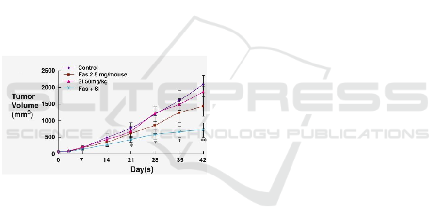
1.2.1 The Target Curve

Figure 1: The target growth curves. We will be bench-

marking our model against the ”control” curve over the ﬁrst

25 days.

We will be bench-marking against the control curve

reported by Chen et al. (Chen et al., ) and shown

in Figure 1, comparing the tumour volume obtained

in our simulation to that obtained in empirical stud-

ies. We will be considering the ﬁrst 2 weeks of tu-

mour growth so as to keep the problem computation-

ally tractable and allow us to repeat large amounts

of simulations on our infrastructure. In picking the

publication we would use as reference, we privileged

those which reported clearly readable growth curves

with a sufﬁcient number of data-points and smaller

error bars.

1.2.2 Spatial Discretization and

Transformations

As mentioned earlier, the environment is discretized

as a Cartesian grid. Table 1 summarizes the effective

sizes of grid positions, alongside other relevant spatial

values such as the volume of cancer cells and initial

tumour volume. Derived 2D values are also reported.

1.2.3 Model Resolution

A decision that needs to be made upfront is the reso-

lution of the model. That is to say, how many cancer

cells will be represented by an agent. This is a com-

promise between model reliability and computational

cost. A high number of cancer cells per agent will

mean overall fewer agents necessary, but lowers the

resolution (Ie: We capture a lower degree of cellu-

lar heterogeneity.), whereas a low number of cancer

cells per agent provides a higher resolution but higher

computational costs. Different resolutions also af-

fect the maximum number of agents per grid position

and the required initial number of agents to achieved

the desired start volume or area. We will be testing

three resolutions: 300, 600 and 1,200 cancer cells per

agent. These are summarized in table 2.

Testing a resolution of fewer than 300 cancer cells

per agent becomes computationally intractable, and

decreasing the resolution to exceed 1,200 cancer cells

per agent results in 2D simulations having a maxi-

mum number of agents per position of 1, which hin-

ders either tumour growth or blood vessel develop-

ment.

1.2.4 Starting Conditions

Cancer cells in an amount appropriate for a given res-

olution are seeded at the center of the grid. Every po-

sition in the grid is seeded with one endothelial cell.

Initial soluble concentrations are calculated and as-

signed to positions. The simulation is thereafter al-

lowed to run its course.

2 RESULTS

Each simulation set (Eg: 300 cancer cells per agent,

2D) comprised 200 simulations. These shared the

same parameters assigned as constant values but dif-

fered in values for those assigned by grid search or

random search and for those related to spatial quanti-

ties such the as maximum number of agents per posi-

tion. Each simulation produced a growth curve which

was compared to an expected growth curve derived

SIMULTECH 2021 - 11th International Conference on Simulation and Modeling Methodologies, Technologies and Applications

242

Table 1: Summary of spatial units for 2D and 3D simulations. 2D values were derived by assuming 3D structures were

cuboids, and then deriving the area of the base. Values are shown to two decimal places.

3D 2D

Item Value Item Value

Volume of Cancer Cell 2,000.00 µm

Area of Cancer Cell 158.74 µm

Volume of Grid Position 0.30 mm

Area of Grid Position 0.45 mm

Start Tumour Volume 1.20 mm

Start Tumour Area 1.13 mm

Table 2: Summary of how different model resolutions affect the maximum number of agents that can be held in a grid position

and the number of agents required at the start to obtain the desired initial volume or area. As expected, increasing the number

of cancer cells per agent decreases both the carrying capacity of individual positions and the initial number of required agents.

Cancer Cells per Agent Max Agents per

Grid Position

Initial Number of

Agents

300

2D 9 24

3D 500 2,000

600

2D 4 12

3D 250 1,000

1,200

2D 2 6

3D 125 500

from medical literature. This gave an indication of the

error rate for such simulation. A set’s performance is

calculated as the average error rate of all simulations

in it. This allows, for each resolution, to compare the

performance of 2D and 3D simulations. For 2D sim-

ulations, an extra step is needed to map areas back to

volumes.

2.1 The Error Function

The aim of the error function is to compare the tu-

mour growth curve produced by a simulation (in-

silico curve) to the one observed in empirical lab-

oratory studies (empirical curve). And ultimately,

to produce a single value: The absolute mean error.

This provides an indication of how closely an in-silico

growth curve aligns to the empirical growth curve.

Expected tumour volumes at different time-points

were estimated from the empirical growth curve (Fig-

ure 1).

A polynomial was then ﬁt to these points describing

the expected volume (V

exp

) at a day (d). This is re-

ported as equation 5, with coefﬁcients reported to two

decimal places.

exp

(d) = 0.95d

+ 18.10d − 65.68; 0 ≤ d ≤ 25 (3)

Given the actual volume at a day d reported in a sim-

ulation’s growth curve, V

act

, then the error ε

is as

reported in equation 4 the magnitude of the difference

between the expected and actual value.

= |V

act

−V

exp

(d)| (4)

The absolute mean error of a simulation (ε) is then

calculated as the average of all errors calculate at each

time-point:

ε = avg(ε

, ε

, ..., ε

d−1

, ε

);0 ≤ d ≤ 25 (5)

2.2 Estimating Volumes from Areas

For 2D simulations, these obviously returned tumour

areas. In order to compare these to expected volumes,

the area was assumed to be the base of a 3D struc-

ture and the corresponding volume was derived via a

simple mathematical transformation.

The generic form of this basic transformation is

provided in equation 6, where V indicates volume and

a area. It represents the derivation of a cube’s volume

from a square’s area by obtaining the square’s width

and raising it to the cube.

V (a) = a

(6)

2.3 Resulting Error Rates

Error rates for 2D and 3D simulations across all res-

olutions are show in ﬁgure 2. For higher resolutions

(Ie: Lower numbers of cancer cells represented by a

single agent), 3D clearly outperforms 2D. At lower

resolutions (Ie: Higher numbers of cancer cells rep-

resented by a single agent) it is the case that the two

approaches appear to be comparable or that 2D out-

performs 3D. This is in fact misleading and will be

addressed in our discussion.

The Trap of 2D in Artiﬁcial Models of Tumours: The Case for 3D In-silico Simulations

243

We note the stability of the error in 3D, where

discrepancies of ±150mm

are owed to the stochas-

tic nature of the model. As for 2D, we note that the

error seems to be linearly dependent and negatively

correlated to the resolution. While it might appear 2D

could be as good as 3D in some instances, this is not

the case and is further elaborated in our discussion.

Finally, a Welch’s t-test was performed compar-

ing the populations of errors for 2D vs. 3D at each

resolution. Results were signiﬁcant for across all res-

olutions for p < 10

−10

. This t-test is appropriate as it

does not assume equal population variance.

3 DISCUSSION

Our results suggest a relatively small and stable er-

ror when it comes to 3D simulations, independently

of the resolution. More interesting is the 2D case,

which seems to outperform 3D at lower resolutions

and whose error seems to increase linearly as resolu-

tion is increased.

This might initially be interpreted as 2D outper-

forming 3D at all but the highest resolutions, suggest-

ing that the former offers a viable if not preferable

alternative to the latter. In fact, such is not the case.

The apparent better performance of 2D is an artifact

of the speciﬁc model conﬁguration which coinciden-

tally allows it to minimize the absolute mean error.

We will discuss how 2D simulations suffer a funda-

mental ﬂaw due to dimensionality mapping from 3D.

We will also emphasize the importance of validation

strategies which go beyond growth curve comparison,

but also consider elements such as soluble concentra-

tions and phenotype ratios within the cancer cell pop-

ulations. Without these additional veriﬁcations our

analysis would be incomplete and lead to the conclu-

sion that 2D forms an alternative to 3D, whereas this

is not the case.

In the ﬁrst instance we note the direction of the

mean error for 2D simulations. Errors are calculated

as the difference between actual and expected vol-

umes. So, a positive error means the model predicted

a larger volume than expected, and a negative one

that the model predicted a smaller volume than ex-

pected. A summary is reported in table 3 (see ap-

pendix). For resolutions of 300 and 600 cancer cells

per agent all simulations consistently over-estimate

tumour growth. For a resolution of 1,200 cancer

cells per agent, a decisive majority of simulation over-

estimates tumour growth. It therefore appears fair to

state that 2D models systematically over-estimate tu-

mour growth.

Given that the magnitude of the error of 2D simula-

tions increases as resolution increases, and that 2D

systematically over-estimate growth, we can say that

as resolution increases 2D simulations over-estimate

growth by larger amounts.

To explain this we need to consider several factors.

First, that as we increase resolution we decrease the

number of cells per agent and therefore we increase

the initial number of agents needed to keep the start-

ing volume consistent. Given more initial agents it

makes sense that the ﬁnal tumour volume should be

greater and that therefore the error should increase,

but this does not explain why we observe this in 2D

but not in 3D.

The reason behind this lies in the effect that 3D

to 2D mapping and resolution adjustments combined

have on the maximum number of agents per position.

In 2D, a position may host between 2 and 9 agents. In

3D, between 125 and 500. (See tables 1 and 2.) This

means that in 3D we may obtain a much higher cancer

to endothelial ratio at each position than in 2D. This

is because cancer cells produce daughter cells each

capable of dividing, resulting in exponential growth,

whereas a tip cell will only produce another tip cell

and trunk cell, the latter being unable to divide, lead-

ing to linear growth.

In both 3D and 2D cancer cells will exceed en-

dothelial cells but, crucially, in 2D space constraints

means the ratio will never increase to the point where

oxygen becomes a limiting factor. This is owed to

the source rate of oxygen being much higher than its

sink rate, and an endothelial cell being able to support

multiple cancer cells. Unless enough space is allowed

at a position for a signiﬁcant amount of cancer cell

divisions, these will never exceed the capacity of the

initial blood vessel network.

In summary, in 2D simulations oxygen never be-

comes a limiting factor of growth meaning that a

higher number of initial cancer cells, as is seeded at

higher resolutions, results in a larger ﬁnal tumour vol-

ume. In 3D instead oxygen may become a limiting

factor and modulates and restricts tumour growth.

Our results raise important considerations for tu-

mour modelling. Where simulations implement a 2D

environment, appropriate scales and parameter values

need to be chosen to avoid issues similar to those we

described which would make the models biologically

implausible. Speciﬁcally, parameter values derived

from 3D studies (such as empirical ones in labora-

tories) should not simply be copied over to 2D in-

silico experiments without consideration being given

to the change of dimensionality. However, publica-

tions rarely discuss the process of deriving their 2D

environments from 3D ones.

Consideration should be given to the use of re-

SIMULTECH 2021 - 11th International Conference on Simulation and Modeling Methodologies, Technologies and Applications

244

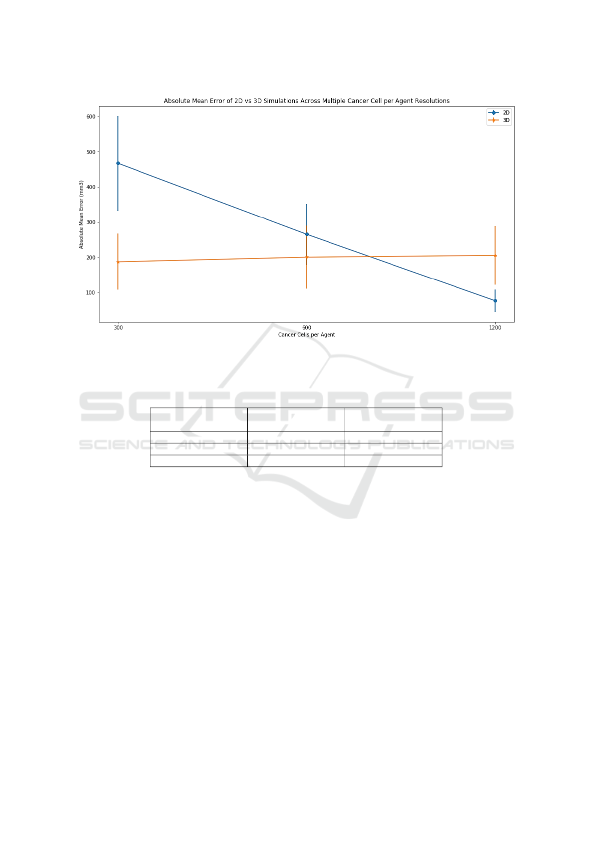
Figure 2: Summary of error rates for each resolution, 2D vs. 3D. Error bars represent standard deviation on the mean. A

higher number of cancer cells per agent indicates a lower resolution, as this means the simulation is modelling larger groups

of cells together rather than allowing them to develop independently.

Table 3: For each resolution we report the number of 2D simulations which over-estimate tumour growth (positive error)

against the number that under-estimate tumour growth (negative error).

Resolution (Cancer

Cells per Agent)

Number of Positive

Errors

Number of Negative

Errors

300 196 0

600 194 0

1,200 187 12

medial action to make 2D models viable. For exam-

ple, by implementing strategies to increase sink rates

or decrease source rates of oxygen. Or, alternatively

and among other possible approaches, decoupling the

maximum number of cells per position from the over-

lying 3D model from which a 2D one has supposedly

been derived. While these approaches may produce

apparently valid results, the question then is what im-

pact does the aforementioned set of remedial actions

have on the reliability of results. For example, setting

the maximum number of agents per cell to an arbi-

trary value may result in a model accepting unrealis-

tic cell concentrations in tissues. Or, tweaking source

and sink values may result in the model working with

hyper- or under-oxygenated tissues.

More importantly, enforcing artiﬁcial constraints

on the model subtracts from its emergent behaviors.

The main value of these models lies in them revealing

unexpected and insightful patterns from a set of sim-

ple, underlying rules. Developers should specify the

behavior of individual agents so that they mimic as

closely as possible their biological counterparts. De-

velopers should not try to direct the evolution of the

model in a speciﬁc direction as they would be doing

when imposing remedial strategies. To do so would

be to constrain the simulation setting it up towards a

speciﬁc conclusion or end-state, which would limit its

usefulness towards gaining additional understanding

of biological phenomena.

It is worth adding some biological considerations

to the limitations of 2D models we discussed. Along-

side unrestricted growth where oxygen is no longer a

limiting factor, other properties of tumours will re-

sult as altered. In 2D we will not observe regions

of hypoxia in the cancer mass, nor the formation of

a necrotic core. Secretion of VEGF will not occur,

which in turn will lead to no angiogenesis or blood

vessel developent. In simulations where these were

implemented, hypoxia-inducible factor (HIF) path-

ways would not be activated. HIF pathways medi-

ate signiﬁcant phenotypic alterations in cancer cells

(Philip et al., 2013; Semenza, 2007), which would

The Trap of 2D in Artiﬁcial Models of Tumours: The Case for 3D In-silico Simulations

245

therefore not be observed in 2D. It is therefore clear

how the impact of oxygen concentrations on 2D mod-

els signiﬁcant affects the accuracy and reliability in a

negative manner.

We also emphasize the numerical scale of our sim-

ulations. Conﬁdence in our results is further rein-

forced by running 200 simulations per simulation set.

(A simulation set refers to, for example, the group

of 2D simulations having 300 cancer cells per agent)

This reduces the likelihood of results being due the

stochastic nature of the model, allowing us to infer

that they are truly representative of the model’s be-

havior.

This contrasts with other publications surveyed,

where the number of simulations run is not discussed.

Given models often include elements of stochastic-

ity, it is important for multiple iterations of these to

be evaluated so as to obtain a clearer picture of their

underlying behavior and evolution. Multiple runs

also allow to explore the search space for parameters

whose value has not been established with certainty,

assessing the model’s sensitivity to changes in these

and informing us about the impact on the results of

the simulation. Search strategies for parametrization,

such as but not limited to grid and random search,

should be explicitly mentioned and discussed. Distri-

bution parameters should be reported, as well as the

number of draws from each distribution and relevant

information. This is necessary for experimental re-

producibility.

We will now consider costs. We ran our sim-

ulations on Amazon AWS EC2 instances of class

r4.large. These feature 2 vCPUs and 16GiB of RAM.

The cost of these is between $0.01 and $0.001 per

hour depending on the speciﬁc plan selected. A sin-

gle 2D simulation took on average one hour and a sin-

gle 3D simulation on average four hours. We will also

note that while we used a large ﬂeet of instances to run

a high number of simulations, individual simulations

could be run in reasonable time within an average of-

ﬁce laptop.

Hence, the price of simulations in 2D or 3D is

comparable. Even for the more expensive 3D simu-

lations, a single simulation set comprising 200 simu-

lations will still cost under $1. Given the severe limi-

tations of 2D we discussed, and the negligible differ-

ences in computational and dollar cost, we think our

investigation makes a very strong case for 3D as the

sole viable solution.

In summary, careless or approximate mapping of

3D environments into 2D ones, or creation of 2D envi-

ronments without consideration for their 3D counter-

parts, raises questions about the validity of the model.

Where this discussion is omitted, as is the case in

many publications, this impacts the reliability of re-

sults as it is not clear what accuracy or resolution has

been achieved by the model. Further, due to the neg-

ligible difference in costs between 2D and 3D, we be-

lieve there is a clear case for the latter to be preferred

over the former.

4 CONCLUSION

We have developed an agent-based model of tumour

growth with continuous elements to account for solu-

ble diffusion and simulated tumour growth in 3D and

derived 2D environments at multiple resolutions of

cancer cells per agent. We have addressed the issue

of parametrization by wherever possible relying on

values in literature, and where these were unknown

using well-established search techniques such as grid

search and random search.

Error rates for each simulation were calculated by

comparing growth curves produced by our model to

those reported in literature, and at each resolution we

compared error distributions and average error val-

ues for 2D and 3D. Initial results suggested, purely

on based on error rates, that 3D simulations consis-

tently produced low error rates and outperformed 2D

at higher resolutions. On the other hand, 2D simula-

tions outperformed 3D at lower resolutions and their

error was dependent on the resolution.

Further analysis revealed that the combined im-

pact of cancer cells per agent resolution and 3D to 2D

mapping signiﬁcantly altered the topology of the 2D

environment. Because of this oxygen concentrations,

a factor limiting growth in 3D, no longer affected tu-

mour growth in 2D. As a result, tumour growth in 2D

became predominantly a function of the initial vol-

ume and was no longer modulated by oxygen avail-

ability as is the case in 3D.

These results highlight the challenges of simulat-

ing a phenomenon that occurs in 3D, such as tumour

growth, in 2D. Neglecting to explicitly derive the 2D

environment from a 3D one, as many publications do,

raises questions about the validity of the model and

realibility of the results.

In conclusion, our results suggest that 3D mod-

els should be preferred to 2D ones. In cases where

3D ones may not be implemented, a clear discussion

should be provided regarding the derivation of the 2D

model from a 3D one.

SIMULTECH 2021 - 11th International Conference on Simulation and Modeling Methodologies, Technologies and Applications

246

REFERENCES

Anderson, a. R. and Chaplain, M. a. (1998). Contin-

uous and discrete mathematical models of tumor-

induced angiogenesis. Bulletin of mathematical biol-

ogy, 60(5):857–899.

Bergstra JAMESBERGSTRA, J. and Yoshua Bengio

YOSHUABENGIO, U. (2012). Random Search for

Hyper-Parameter Optimization. Journal of Machine

Learning Research, 13:281–305.

Cai, Y., Wu, J., Li, Z., and Long, Q. (2016). Mathematical

Modelling of a brain tumour initiation and early de-

velopment: A coupled model of glioblastoma growth,

pre-existing vessel co-option, angiogenesis and blood

perfusion. PLoS ONE, 11(3):1–28.

Cai, Y., Xu, S., Wu, J., and Long, Q. (2011). Coupled

modelling of tumour angiogenesis, tumour growth

and blood perfusion. Journal of Theoretical Biology,

279(1):90–101.

Chen, Y., Alvarez, E. A., Azzam, D., Wander, S. A., Gug-

gisberg, N., Jord

a, M., Ju, Z., Hennessy, B. T., and

Slingerland, J. M. Combined Src and ER blockade

impairs human breast cancer proliferation in vitro and

in vivo.

Duval, K., Grover, H., Han, L. H., Mou, Y., Pegoraro, A. F.,

Fredberg, J., and Chen, Z. (2017). Modeling physio-

logical events in 2D vs. 3D cell culture.

Gabhann, F. M., Ji, J. W., and Popel, A. S. Computational

Model of Vascular Endothelial Growth Factor Spatial

Distribution in Muscle and Pro-Angiogenic Cell Ther-

apy.

Guyer, J. E., Wheeler, D., and Warren, J. A. (1988). FiPy:

Partial Differential Equations with Python. Comput-

ing in Science Engineering, 11(3):6–15.

Hoarau-V

echot, J., Raﬁi, A., Touboul, C., and Pasquier,

J. (2018). Halfway between 2D and animal mod-

els: Are 3D cultures the ideal tool to study cancer-

microenvironment interactions?

Imamura, Y., Mukohara, T., Shimono, Y., Funakoshi, Y.,

Chayahara, N., Toyoda, M., Kiyota, N., Takao, S.,

Kono, S., Nakatsura, T., and Minami, H. (2015).

Comparison of 2D- and 3D-culture models as drug-

testing platforms in breast cancer. Oncology Reports,

33(4):1837–1843.

Lv, D., Hu, Z., Lu, L., Lu, H., and Xu, X. (2017). Three-

dimensional cell culture: A powerful tool in tumor re-

search and drug discovery.

Melissaridou, S., Wiechec, E., Magan, M., Jain, M. V.,

Chung, M. K., Farnebo, L., and Roberg, K. (2019).

The effect of 2D and 3D cell cultures on treatment

response, EMT proﬁle and stem cell features in head

and neck cancer 11 Medical and Health Sciences 1112

Oncology and Carcinogenesis. Cancer Cell Interna-

tional, 19(1).

Olsen, M. M. and Siegelmann, H. T. (2013). Multiscale

agent-based model of tumor angiogenesis. Procedia

Computer Science, 18:1016–1025.

Philip, B., Ito, K., Moreno-S

anchez, R., and Ralph, S. J.

(2013). HiF expression and the role of hypoxic mi-

croenvironments within primary tumours as protective

sites driving cancer stem cell renewal and metastatic

progression. Carcinogenesis, 34(8):1699–1707.

Pickl, M. and Ries, C. H. (2009). Comparison of 3D

and 2D tumor models reveals enhanced HER2 acti-

vation in 3D associated with an increased response to

trastuzumab. Oncogene, 28(3):461–468.

Riedl, A., Schlederer, M., Pudelko, K., Stadler, M., Wal-

ter, S., Unterleuthner, D., Unger, C., Kramer, N.,

Hengstschl

ager, M., Kenner, L., Pfeiffer, D., Krupitza,

G., and Dolznig, H. (2017). Comparison of cancer

cells in 2D vs 3D culture reveals differences in AKT-

mTOR-S6K signaling and drug responses. Journal of

Cell Science, 130(1):203–218.

Rios, L. M., Nikolaos, ·., Sahinidis, V., and Rios, L. M.

(2013). Derivative-free optimization: a review of

algorithms and comparison of software implementa-

tions. J Glob Optim, 56:1247–1293.

Semenza, G. L. (2007). HIF-1 mediates the Warburg effect

in clear cell renal carcinoma. Journal of Bioenergetics

and Biomembranes, 39(3):231–234.

Shirinifard, A., Gens, J. S., Zaitlen, B. L., Popławski, N. J.,

Swat, M., and Glazier, J. A. (2009). 3D multi-cell

simulation of tumor growth and angiogenesis. PLoS

ONE, 4(10).

Sinek, J., Frieboes, H., Zheng, X., and Cristini, V. (2004).

Two-dimensional chemotherapy simulations demon-

strate fundamental transport and tumor response limi-

tations involving nanoparticles. Biomedical Microde-

vices, 6(4):297–309.

Skeldon, A. C., Chaffey, G., Lloyd, D. J., Mohan, V.,

Bradley, D. A., and Nisbet, A. (2012). Modelling

and detecting tumour oxygenation levels. PLoS ONE,

7(6):1–29.

St, A., ˜phanou, ., Mcdougall, S. R., Anderson, A. A. A.,

and Chaplain, M. A. J. (2005). MATHEMATI-

CAL AND Mathematical Modelling of Flow in 2D

and 3D Vascular Networks: Applications to Anti-

Angiogenic and Chemotherapeutic Drug Strategies.

COMPUTER MODELLING Mathematical and Com-

puter Modelling, 41:1137–1156.

Sun, X., Zhang, L., Tan, H., Bao, J., Strouthos, C., and

Zhou, X. (2012). Multi-scale agent-based brain cancer

modeling and prediction of TKI treatment response:

Incorporating EGFR signaling pathway and angiogen-

esis. Technical report.

Turner, S. and Sherratt, J. A. (2002). Intercellular adhesion

and cancer invasion: A discrete simulation using the

extended potts model. Journal of Theoretical Biology,

216(1):85–100.

Zhang, L., Jiang, B., Wu, Y., Strouthos, C., Zhe Sun, P.,

Su, J., and Zhou, X. (2011). Developing a multi-

scale, multi-resolution agent-based brain tumor model

by graphics processing units. Technical report.

The Trap of 2D in Artiﬁcial Models of Tumours: The Case for 3D In-silico Simulations

247