Guided Bee Colony Algorithm Applied to the Daily Car Pooling Problem

Mouna Bouzid, Ines Alaya and Moncef Tagina

LARIA-ENSI, National School of Computer Sciences, University of Manouba, Manouba 2010, Tunisia

Keywords:

Metaheuristic, Bee Colony Optimization, The Daily Car Pooling Problem.

Abstract:

The foraging behavior of bees has been adapted in a Bee Colony Optimization algorithm (BCO). This approach

is a simple and an efﬁcient metaheuristic that has been successfully used to solve many complex optimization

problems in different domains, mostly in transportation, location and scheduling ﬁelds.

In this study, we develop two algorithms for the Daily Car Pooling Problem based on the BCO approach. The

developed algorithms are experimentally tested on benchmark instances of different sizes. The computational

results show that the proposed approaches can produce good solutions when compared with an exact method.

1 INTRODUCTION

In recent decades, the increased human mobility and

the high use of private vehicles has caused many prob-

lems, such as air pollution, parking problem, trafﬁc

congestion, noise pollution, toxic emissions, and in-

crease in the number of crashes and accidents.

Public transportation service can be a solution to

this problem but it cannot adequately cover all pas-

senger transportation needs. Car pooling has emerged

to be another solution for reducing private car usage

around the world.

Car pooling (Bruglieri et al., 2011; Manzini and

Pareschi, 2012; Correia and Viegas, 2011; Yan et al.,

2011; Vargas et al., 2008) is a collective transportation

system that encourage people to share a common car

to reach the same destination, in order to decrease the

number of cars on the road.

In literature, we distinguish two main ways of op-

erating the car pooling. It can be either a Daily Car

Pooling Problem (DCPP) or a Long-Term Car Pool-

ing Problem (LTCPP).

In the case of DCPP (Baldacci et al., 2004; Calvo

et al., 2004; Swan et al., 2013), on each day a number

of users (servers) are available to share their vehicle

with colleagues (clients) on that particular day. The

problem is to assign clients to servers and to iden-

tify the routes to be driven by the servers. The aim

is to minimize the total travel cost, with respect to

time window and car capacity constraints. The DCPP

can be considered as a special case of the Dial-a-

Ride Problem (DARP) or the Vehicle routing problem

(VRP). The DCPP is a NP-hard problem as it is a spe-

cial case of the VRP which is known to be NP- hard

Problem (Toth and Vigo, 2014).

However, in the case of LTCPP (Guo et al., 2012;

Yan et al., 2011; Bouzid et al., 2020), each user is

available to act both as a server and as a client. The

LTCPP requires to deﬁne crews — or user pools —

where each user will in turn, on different days, pick up

the remaining pool members. The objective here be-

comes that of maximizing pool sizes and minimizing

the total distance travelled by all users when acting

as servers, subject to car capacity and time window

constraints.

The speciﬁc problem addressed in this paper is the

DCPP. In spite of its hardness, only few researches

have been carried out in this problem.

Authors in (Baldacci et al., 2004) present both an

exact and a heuristic method for the DCPP based on

two integer programming formulations of the prob-

lem. The exact method is based on a bounding proce-

dure that combines three lower bounds derived from

different relaxations of the problem. A valid upper

bound is obtained by the heuristic method, which

transforms the solution of a Lagrangean lower bound

into a feasible solution.

In (Calvo et al., 2004), Calvo et al. give another al-

gorithm solving the DCPP. The main idea of this algo-

rithm is the use of greedy assignment alternating with

random perturbation. In fact, the greedy assignment

phase look to minimize a marginal quantity called re-

gret. Where the regret for each client i is given by the

difference of the length paths between the two servers

which have the least and the second least extra mile

when pick up client i.

Bouzid, M., Alaya, I. and Tagina, M.

Guided Bee Colony Algorithm Applied to the Daily Car Pooling Problem.

DOI: 10.5220/0010517504650472

In Proceedings of the 16th International Conference on Software Technologies (ICSOFT 2021), pages 465-472

ISBN: 978-989-758-523-4

465

Authors in (Swan et al., 2013) examine the effect

of varying the acceptance criterion. In particular, they

investigate the use of Late-acceptance Hillclimbing.

In this metaheuristic a new solution is accepted if it is

no worse than the k-th most recent solution.

After bibliographical study, we remarked that the

Bee Colony Optimization algorithm has been used

only to solve the LTCPP. Authors in (Bouzid et al.,

2020) developed a Bee Colony Optimization algo-

rithm for the Long-term Car Pooling problem where

all choices in back-ward pass are random.

In this article, we present a different algorithm

based on the Bee Colony Optimization to solve the

second type of car pooling: the Daily Car pooling

problem. In this algorithm, called the Guided-BCO

algorithm, all choices in the back-ward pass are based

on probability equations. This algorithm is com-

pared with an exact method (Baldacci et al., 2004)

and tested on two classes of benchmark instances

from (Christoﬁdes and Eilon, 1969; Christoﬁdes,

1979; Fisher, 1994). We have also developed another

version of BCO algorithm where all decisions and

choices in the backward pass are random, named Ran-

dom BCO-DCPP algorithm and we have compared

this version with the Guided BCO algorithm.

The paper introduces an adaptation of the Bee

Colony Algorithm (BCO) to the Daily Car Pooling

Problem ( DCPP) and it is organized as follows. The

DCPP, whose target is to share vehicles among users

(servers and clients ) to minimize the total travel cost

is expressed in Section 2. The BCO, in which an

artiﬁcial bee colony visits the search space to ﬁnd

a feasible solution, is described in Section 3. BCO

is adapted to DCPP, by specializing the forward and

backward phases of BCO, in Section 4. Experimental

results and comparisons are the focus of Section 5.

2 PROBLEM FORMULATION

In this section, we present a mathematical formulation

of the DCPP using research in (Baldacci et al., 2004).

Mathematically, the DCPP can be described by

a directed graph G = {V ∪ {0},A}, where V =

{1,. . . ,n} is the set of employees, 0 represents the

destination, and A = {arc(i, j)/i ∈ V, j ∈ V ∪ {0}}

is the set of arcs. Every arc (i, j) ∈ A is associated

with a non-negative travel cost d

i j

and a travel time

i j

. Each employee i ∈ V is speciﬁed by an origin

(home), a node 0 represents the destination, a non-

negative value representing the earliest departure time

for leaving home; and a positive value denoting the

acceptable time l

for arriving at destination. The set

V is partitioned as V = V

∪V

, where V

= {1,...,n

}

is the subset of servers and V

= {n

+ 1, . . . ,n} is the

subset of clients. For each server k ∈ V

, we denote

by Q

the car capacity and by T

the maximum driv-

ing time he is willing to go from home to workplace.

Each client i ∈ V

is characterized by a penalty p

rep-

resenting its contribution to the total cost in case no

server picks him up. We denote by Γ

= { j : (i, j) ∈ A}

the set of successors of vertex i ∈ V ∪ {0}, and by

−1

= {i : (i, j) ∈ A} the set of predecessors.

Before formulate our problem, we should present

some notations:

• x

i j

: Binary variable equals to 1 if and only if arc

(i,j) is traveled by a server k, with (i, j) ∈ A and

k ∈ V

• y

: Binary variable equals to 1 if and only if i is

not picked by any server, where k ∈ V

and i ∈ V

• S

: Positive variable indicating the pick-up time

of employee i ∈ V .

• h

: Non-negative variable denoting the arrival

time of server k ∈ V

at the destination.

Objective function:

MinZ(F) =

∑

(k∈V

)

∑

(i, j)∈A

i j

∑

i∈V

(1)

Constraints :

∑

j∈Γ

k j

= 1; k ∈ V

; (2)

∑

j∈Γ

−1

= 1; k ∈ V

; (3)

∑

j∈Γ

−1

−

∑

j∈Γ

i j

= 0; k ∈ V

,i ∈ V

; (4)

∑

(i, j)∈A

i j

≤ Q

;k ∈ V

; (5)

∑

(i, j)∈A

i j

≤ T

;k ∈ V

; (6)

− S

≥ t

i j

+ M(1 −

∑

k∈V

i j

);(i, j) ∈ A; (7)

≥ e

;i ∈ V, (8)

≥ S

− M(1 − x

);i ∈ V, k ∈ V

; (9)

≤ l

+ M(1 −

∑

j∈Γ

i j

);i ∈ V, k ∈ V

; (10)

∑

k∈V

∑

j∈Γ

i j

+ y

= 1; i ∈ V

(11)

i j

∈ {0,1}; (i, j) ∈ A, k ∈ V

, (12)

∈ {0,1}; i ∈ V

; (13)

≥ 0; k ∈ V

; (14)

≥ 0; i ∈ V ; (15)

ICSOFT 2021 - 16th International Conference on Software Technologies

466

Equation (2) shows that every server must leave its

house and equation (3) forces it to arrive at the des-

tination (workplace). Constraint (4) makes sure the

continuity of the path. The capacity and the maxi-

mum time constraints are translated in inequalities (5)

and (6), respectively. Equations (7) and (8), where M

is a big constant, deﬁne the arrival time variables S

while inequalities (9) and (10) set the arrival times h

, k ∈ V

, of the servers at the workplace and assume

that each employee i ∈ V should reach the workplace

before the latest arrival time l

, respectively. Equa-

tion (11) ensures that each client can be picked by a

server or is left unserved. Constraints (12) and (13)

are binary constraints, while (14) and (15) are posi-

tivity constraints.

3 THE BEE COLONY

OPTIMIZATION ALGORITHM

The Bee Colony Optimization is among the famous

natural inspired metaheuristic based on the collective

bee intelligence. It was proposed, ﬁrst, by Lucic and

Teodorovic (Lu

c and Teodorovi

c, 2003) to deal with

the well hard combinatorial optimization problems

like the Vehicle Routing Problem (Lu

c and Teodor-

ovi

c, 2003; Teodorovi

c, 2008), the Job Shop Schedul-

ing Problem (Chong et al., 2006; Chong et al., 2007),

the p-Median Problem (Teodorovic and

Selmic, 2007)

and the Traveling Salesman Problem (Wong et al.,

2010).

The main idea of this approach is to build an ar-

tiﬁcial bee colony, where bees investigate through

the search space looking for feasible solutions. Af-

ter that, they communicate, collaborate and exchange

information. Thanks to this communication systems

named ”Swarm Intelligence”, and using collective

knowledge and information sharing, artiﬁcial bees in-

crementally construct solution to the problem. The

BCO performs its search process in iterations until a

stopping condition is met.

Flying through the space, an artiﬁcial bee per-

forms either forward pass or backward pass. In

the case of forward pass, every bee makes a prede-

ﬁned number of local moves, which slowly construct

and/or improve the solution, yielding a new solution.

Building partial solutions, bees start the second phase

called the backward pass. In this phase, bees return to

the hive. They exchange information about the qual-

ity of the partial solution created which is deﬁned as

the current value of the objective function.

Having the evaluation of all partial solutions, each

bee decides with a certain probability whether to still

faithful to its created partial solution or not. It is obvi-

ous that bees with better solutions have greater chance

to keep and continue their own exploration.

Faithfull bees are considered as recruiters, and

their solutions would be considered by other bees.

However, if a bee chooses to abandon its solution it

becomes uncommitted and it has to select one solu-

tion from recruiters by the roulette wheel. Note that

better solutions have higher opportunities to be cho-

sen for further exploration. Forward and backward

pass, could be iteratively performed until each bee

completes the generation of its solution or a stopping

condition is satisﬁed. Among the possible stopping

conditions, we found the maximum total number of

forward/backward passes or the maximum total num-

ber of forward/backward passes without the improve-

ment of the objective function, etc.

4 THE PROPOSED BCO

ALGORITHM FOR THE DCPP

In this section, we present our algorithm based on the

Bee Colony Optimization called the Guided-BCO al-

gorithm.

4.1 Problem Representation

In order to maintain the simplicity of the BCO algo-

rithm, a rather straightforward solution representation

scheme is adopted. Let us represent each employee

by a node. Our problem is divided into stages where

the ﬁrst stage represents servers and all others repre-

sent clients. In every stage, an artiﬁcial bee chooses

to visit one node. At the beginning of each new pool,

the selection of a new server (new initial node) was

represented by changing the location of a hive.

4.2 Forward Pass Phase

At the beginning of the BCO process, all artiﬁcial

bees are located in the hive. Bees depart from the

hive and ﬂy to an unvisited client who satisﬁes con-

straints. It chooses a new node to be added to his

partial pool using the roulette wheel selection. This

technic is based on the probability values, which gives

the bee the likelihood to move from client i to client

j. To calculate the probability, we need the distance

between the current client i and the client to be vis-

ited j. It is obvious that, the shorter the distance,

the higher the probability to choose a client. There-

fore, the travel cost and the probability are inversely

proportional. Formally, the probability is deﬁned in

equation (16) as follow:

Guided Bee Colony Algorithm Applied to the Daily Car Pooling Problem

467

i j

∑

j∈V

i j

(16)

4.3 Backward Pass Phase

During the backward pass, bees evaluate the quality of

all generated partial solutions by calculating the cur-

rent value of the objective function using equation (1).

Then, each bee b decides whether to stay loyal to its

partial solution or to abandon it. This choice was per-

formed in a probabilistic manner. This probability is

expressed as follows:

u+1

= e

−

max

−O

;b = 1,2,..., B (17)

Where:

• O

max

: denotes the maximum over all normalized

values of partial/complete solutions to be com-

pared;

• O

: represents the normalized value for the objec-

tive function of partial/complete solution created

by the b-th bee;

• U: is the number of forward pass;

Since we are in the case of minimization criterion, the

normalized value is calculated as follows:

max

−C

max

−C

min

;b = 1,2,.., B (18)

Where:

• C

: is the value for the objective function of b-th

bee partial/ complete solution;

• C

min

: represents the minimal objective function

value obtained by all engaged bees;

• C

max

: denotes the maximal objective function

value obtained by all engaged bees;

Using a random number and equation (17) each bee

can make its decision. In fact, if the generated num-

ber is greater than the calculated probability the bee

is considered uncommitted else it is considered re-

cruiter. Once the bee becomes uncommitted, it must

choose which recruiter it will follow by the roulette

wheel. Also, this selection is guided by a probabil-

ity. The probability that b’s partial/complete solution

would be chosen by any uncommitted bee is equal to:

∑

k=1

;b = 1,2,..., R; (19)

Where O

is the normalized value for the objective

function of the k-th solution and R denotes the num-

ber of recruiters.

4.4 Solution Construction

In order to build a pool, the two steps of the search al-

gorithm, forward and backward pass, are alternated it-

eratively until the total number of forward/ backward

passes reaches the car pool size. At this point, the

best among all B pools is determined. It is then used

to build a global solution and the construction of a

new pool begins. The iteration is considered ﬁnished,

when all clients are assigned to servers. Our algo-

rithm runs iteration by iteration until the maximum

number of iterations is reached. At the end, the global

best-found solution is reported as the solution of our

problem.

4.5 Guided BCO-DCPP Algorithm

The overall structure of the Guided BCO-

DCPP is outlined as shown in Algorithm 1.

Algorithm 1: Guided BCO-DCPP Algorithm.

Initialize parameters:- Number of bees B.

- Number of iterations.

Repeat

For every server i in the set of servers do{

Initialization: every bee is set to an empty pool;

Add server i to every pool;

While the car capacity of server i is not reached

do{

Forward pass

a) For every bee do {

i. Evaluate all unserved clients in the current

set of clients not yet pooled;

ii. Choose an unserved client c who satisﬁes

constraints using the roulette wheel selection

based on equation (16);

iii. Insert client c into the current car pool

and eliminate it from the current set of

clients not yet pooled;}

Backward pass

b) For every bee do {

Evaluate partial pool using equation (1); }

c) For every bee do {

Loyalty decision using equation (17); }

d) For every uncommitted bee do {

Choose a recruiter bee to follow by a roulette

selection based in equation (19); } }

Evaluate all pools, ﬁnd the best one and add it to

the current partial solution; }

Update the best solution;

Until the number of iteration is reached;

Out put the best solution;

ICSOFT 2021 - 16th International Conference on Software Technologies

468

5 EXPERIMENTAL STUDY AND

DISCUSSION

In order to improve the performance and the efﬁ-

ciency of our proposed algorithm and after biblio-

graphic research we have chosen to compare our ap-

proach with the exact algorithm described in (Bal-

dacci et al., 2004) since there aren’t other intelligent

algorithms carried out on this problem.

Also, we have developed another version of BCO

algorithm where all decisions and choices in the back-

ward pass are random, that is why it is named a Ran-

dom BCO-DCPP algorithm and we have compared

this version of algorithm with the Guided BCO algo-

rithm.

5.1 Benchmarks

We have tested both the Random BCO and the Guided

BCO algorithms on two classes of benchmark in-

stances: Class A and Class B. Class A includes in-

stances originally derived from dataset provided by

Christoﬁdes and Eilon (1969) (Christoﬁdes and Eilon,

1969), Christoﬁdes et al. (1979) (Christoﬁdes, 1979)

and Fisher (1994) (Fisher, 1994) for the VRP. The

number of users in each instance is ranging from 51

to 225.

For all instances of class A, we considered the

depot as the destination, while we retained the co-

ordinates of the customers, who become the employ-

ees. We randomly choose n/4 among employees to be

considered as servers of our problem (n

= n/4) and

others are considered as clients. The cost d

i j

was as-

sumed to be equal to the Euclidean distance between

user i and j. The travel time t

i j

were set to be equal to

the distance d

i j

For each server k ∈ V

, the car capacity Q

was set

with equal probability to be equal to 4 or 5 and the

maximum ride time T

was calculated as T

= 1.5t

where t

is the time needed to travel from the server

k’s home to the destination.

For each client i ∈V

, the penalty p

was computed

as p

= 2d

, where d

is the travel cost from client’s

home directly to the destination.

The latest arrival times l

is an integrate value ran-

domly selected in the interval [510, 540], and the ear-

liest departure time e

was estimated to be equal to

= l

–max(t

+ 30, 2t

), with i ∈ V .

Class B contains 23 problems composed of users

ranging from 50 to 250. This class of instance is

selecting from the real-world instance for a research

institution in Italy. In fact, the car capacity Q

, the

maximum ride time T

(k ∈ V

), the penalty p

(i ∈ V

the latest arrival times l

, the earliest departure time e

(i ∈ V ) are calculated exactly like in the class A.

5.2 Parameters Setting

All computational results were obtained on a 3317U,

1.70 GHz computer, and the proposed algorithms

were coded in java.

For the experiments, some common parameters

were set as follows:

- Number of iterations: IT = 1000,

- Number of bees: B = number of users of the in-

stance.

5.3 Comparative Results

In this section, we evaluate the developed algorithms

by comparing them with the exact algorithm. The re-

sults of the exact algorithm are gained directly from

(Baldacci et al., 2004). We run both algorithms 30

times for each instance.

Tables 1 and 2 present a summary result of our

study. For each test instance, the table indicates the

number of employees n, the number of servers n

, the

number of clients n

, the optimal solution value found

by the exact algorithm. We also report the best (Best)

and the average (AVG) values obtained by the devel-

oped algorithms. In addition, tables give the deviation

(DV%) of best BCO from the optimal solution. Fur-

thermore, to validate the statistical signiﬁcance of the

proposed algorithms we have use the non-parametric

Wilcoxon rank signed test (Sheskin, 2003) (W-test).

Note that for W-Test, the level of signiﬁcance con-

sidered is 0.05. We use (+) and (-) to denote if the

Guided BCO results, respectively, signiﬁcantly or not

signiﬁcantly better than the Random BCO algorithm.

Table 1 summarizes the results of instances of

class A. Through this table, we can say that the aver-

age deviation of the best solution for the Guided BCO

from the optimal solution is 0.43% and that the av-

erage deviation of the best solution for the Random

BCO from the optimal solution is 0.89%. So, we can

say that both algorithms can produce good results.

Indeed, the Guided BCO algorithm outperforms the

Random algorithm in 11 instances from 12 instances

in average solution and in the best-found solution.

Also, statistically, the Guided BCO algorithm is sig-

niﬁcantly better than the Random BCO algorithm in

ten instances among the twelve instances.

Guided Bee Colony Algorithm Applied to the Daily Car Pooling Problem

469

Table 1: Comparison of Guided BCO and Random BCO algorithms with the exact method on set A instances.

Exact method Guided BCO Random BCO W-test

Instance n n

Optimal Best AVG DV% Best AVG DV%

A1 51 13 37 1202 1210 1237.5 0.67 1213 1241.4 0.92 (+)

A2 76 19 56 1490 1493 1526.5 0.2 1496 1547.67 0.4 (+)

A3 101 26 74 1378 1386 1461.75 0.58 1390 1479.5 0.87 (+)

A4 121 31 89 2348 2356 2389.6 0.34 2410 2453.86 2.64 (+)

A5 121 31 89 1949 1960 2010.14 0.56 1975 2014.36 1.33 (+)

A6 135 34 100 2271 2288 2325.26 0.75 2311 2415.23 1.76 (+)

A7 151 38 112 2091 2092 2118.72 0.05 2094 2152.37 0.14 (+)

A8 171 43 127 2872 2882 2922.67 0.35 2881 2923.88 0.31 (-)

A9 171 43 127 2668 2681 2738.38 0.49 2689 2759.37 0.79 (+)

A10 196 49 146 3187 3190 3232.25 0.09 3195 3231.17 0.25 (-)

A11 200 50 149 2355 2376 2417.35 0.89 2381 2454.29 1.1 (+)

A12 226 57 168 2343 2346 2377.46 0.13 2347 2396.12 0.17 (+)

Average 2179.5 2188.33 2229.8 0.43 2198.5 2255.77 0.89

Table 2: Comparison of Guided BCO and Random BCO algorithms with the exact method on set B instances.

Exact method Guided BCO Random BCO W-test

Instance n n

Optimal Best AVG DV% Best AVG DV%

B1 101 25 75 1509 1511 1521.5 0.13 1512 1548.6 0.2 (+)

B2 101 25 75 1484 1501 1537.2 1.35 1542 1573.71 3.9 (+)

B3 101 25 75 1445 1465 1496.7 1.38 1471 1499.3 1.8 (+)

B4 101 25 75 2218 2246 2266.14 1.26 2259 2273.21 1.85 (+)

B5 101 25 75 1593 1594 1627.34 0.06 1602 1640.53 0.56 (+)

B6 101 25 75 1282 1287 1298.42 0.39 1288 1300.86 0.47 (+)

B7 101 25 75 1333 1348 1371.87 1.12 1336 1377.42 0.23 (+)

B8 151 38 112 1985(a) 1799 1836.5 -9.37 1784 1817.13 -10.13 (-)

B9 151 38 112 1970 1998 2018.33 1.42 2016 2020.86 2.34 (+)

B10 151 38 112 2560(a) 2422 2453.16 -5.39 2431 2459.43 -5.03 (+)

B11 151 38 112 2010(a) 1867 1913.33 -7.11 1909 1951.11 -5.02 (+)

B12 151 38 112 1674 1687 1698.83 0.78 1693 1705.14 1.13 (+)

B13 201 50 150 2467(a) 2307 2335.11 -6.49 2309 2342.8 -6.4 (+)

B14 201 50 150 2289(a) 1807 1868.77 -21.06 1801 1862.2 -21.32 (-)

B15 201 50 150 3109(a) 2903 2943.1 -6.63 2957 2978.7 -4.89 (+)

B16 201 50 150 3172(a) 2927 2977.7 -7.72 3026 3048.5 -4.6 (+)

B17 201 50 150 3660(a) 3413 3435.89 -6.75 3410 3439.3 -6.83 (+)

B18 201 50 150 2521(a) 2386 2416.1 -5.36 2436 2480.9 -3.37 (+)

B19 251 63 187 3244(a) 3012 3040.25 -7.15 3011 3044.34 -7.18 (+)

B20 251 63 187 3312 3316 3336.34 0.12 3318 3339.55 0.18 (+)

B21 251 63 187 3676 3680 3690.12 0.11 3678 3689.32 0.05 (+)

B22 251 63 187 3323 3325 3348.11 0.06 3324 3351.33 0.03 (+)

B23 251 63 187 3000 3049 3079.3 1.63 3057 3083.56 1.9 (+)

Average 2139.92 2297.83 2326.53 -3.18 2311.74 2340.34 -2.61

Note. (a) Instances that had not been solved to optimality by Maniezzo.

From table 2, we can easily see that the Guided

BCO algorithm gets the best solution on 16 instances

from 23 and on 20 instances considering the average

solution quality comparing with the Random BCO al-

gorithm. Moreover, the average deviation percentages

for all set B instances are -3.18% for Guided BCO

and -2.61% for Random BCO from exact method.

Here, it should be noted that instances B8, B10, B11,

B13, B14, B15, B16, B17, B18 and B19 had not

been solved to optimality by Maniezzo. It means that

our proposed algorithms are more robust and more

efﬁcient for these ten instances and that these algo-

ICSOFT 2021 - 16th International Conference on Software Technologies

470

rithms can produce very good solutions for all set B

instances. Remarkably, the Guided BCO algorithm is

signiﬁcantly better than the Random BCO on 21 in-

stances of class B.

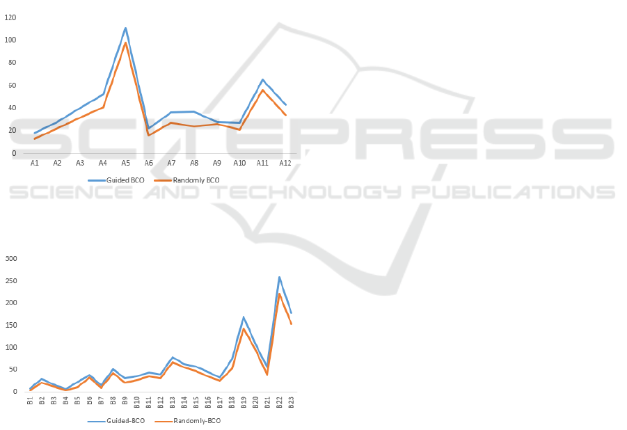
5.4 Comparison of Execution Times of

Guided BCO with Random BCO

The time taken to execute the proposed algorithms is

given in ﬁgure 1 and ﬁgure 2. Both algorithms were

executed on the same machine.

Based on ﬁgure 1 and ﬁgure 2 we can state that

for all instances the Random BCO algorithm curve is

always above the Guided BCO curve. So, we can con-

clude that the Random BCO algorithm requires very

little execution time and it is slightly more quickly

than the Guided BCO on all instances of different

classes.

Figure 1: Computing time needed by the Guided BCO al-

gorithm and the Random BCO algorithm for instances of

class A (in seconds).

Figure 2: Computing time needed by the Guided BCO al-

gorithm and the Random BCO algorithm for instances of

class B (in seconds).

All in all, we can say that the Guided BCO algo-

rithm outperforms the Random BCO algorithm, even

if it takes very slightly more CPU time.

6 CONCLUSIONS

In this paper, we presented two different intelligent

algorithms inspired from bee’s behavior to solve the

Daily Car Pooling Problem, one is called the Guided

BCO algorithm and the other is named the Random

BCO algorithm. To show the effectiveness of the de-

veloped algorithms we have tested them on different

benchmark instances. Experimental results show that

developed algorithms can produce very good results.

To the best of our knowledge, these are the ﬁrst swarm

intelligent algorithms solving the DCPP.

These results motivate us to apply the proposed

BCO algorithm on other similar problems like vehicle

routing problem or travelling thief problem.

REFERENCES

Baldacci, R., Maniezzo, V., & Mingozzi, A. (2004). An

exact method for the car pooling problem based on

lagrangean column generation. Operations Research,

52(3), 422-439.

Bouzid, M., Alaya, I., & Tagina, M. (2020). A Bee Colony

Optimization Algorithm for the Long-Term Car Pool-

ing Problem. In 15th International Conference on

Software Technologies (ICSOFT 2020).

Bruglieri, M., Ciccarelli, D., Colorni, A., & Lu

e, A. (2011).

PoliUniPool: a carpooling system for universities.

Procedia-Social and Behavioral Sciences, 20, 558-

567.

Calvo, R. W., de Luigi, F., Haastrup, P., & Maniezzo, V.

(2004). A distributed geographic information system

for the daily car pooling problem. Computers & Op-

erations Research, 31(13), 2263-2278.

Chong, C. S., Low, M. Y. H., Sivakumar, A. I., & Gay, K.

L.(2006, December). A bee colony optimization algo-

rithm to job shop scheduling. In Proceedings of the

2006 winter simulation conference (pp. 1954-1961).

IEEE.

Chong, C. S., Low, M. Y. H., Sivakumar, A. I., & Gay, K.

L. (2007). Using a bee colony algorithm for neigh-

borhood search in job shop scheduling problems. In

21st European conference on modeling and simula-

tion (ECMS 2007).

Christoﬁdes, N. (1979). The vehicle routing problem. Com-

binatorial optimization.

Christoﬁdes, N., & Eilon, S. (1969). An algorithm for the

vehicle-dispatching problem. Journal of the Opera-

tional Research Society, 20(3), 309-318.

Correia, G., & Viegas, J. M. (2011). Carpooling and car-

pool clubs: Clarifying concepts and assessing value

enhancement possibilities through a Stated Preference

web survey in Lisbon, Portugal. Transportation Re-

search Part A: Policy and Practice, 45(2), 81-90.

Fisher, M. L. (1994). Optimal solution of vehicle rout-

ing problems using minimum k-trees. Operations re-

search, 42(4), 626-642.

Guided Bee Colony Algorithm Applied to the Daily Car Pooling Problem

471

Guo, Y. (2012). Metaheuristics for solving large size long-

term car pooling problem and an extension.

c, P., & Teodorovi

c, D. (2003). Vehicle routing problem

with uncertain demand at nodes: the bee system and

fuzzy logic approach. In Fuzzy sets based heuristics

for optimization (pp. 67-82). Springer, Berlin, Heidel-

berg.

Manzini, R., & Pareschi, A. (2012). A decision-support sys-

tem for the car pooling problem. Journal of Trans-

portation Technologies, 2(02), 85.

Sheskin, D. J. (2003). Handbook of parametric and non-

parametric statistical procedures. crc Press.

Swan, J., Drake, J.,

Ozcan, E., Goulding, J., & Woodward,

J. (2013). A comparison of acceptance criteria for the

daily car-pooling problem. In Computer and informa-

tion sciences III (pp. 477-483). Springer, London.

Teodorovi

c, D. (2008). Swarm intelligence systems for

transportation engineering: Principles and applica-

tions. Transportation Research Part C: Emerging

Technologies, 16(6), 651-667.

Teodorovic, D., &

Selmic, M. (2007). The BCO algorithm

for the p-median problem. Proceedings of the XXXIV

Serbian Operations Research Conferece, 417-420.

Toth, P., & Vigo, D. (Eds.). (2014). Vehicle routing: prob-

lems, methods, and applications. Society for Industrial

and Applied Mathematics.

Vargas, M. A., Sefair, J., Walteros, J. L., Medaglia, A. L., &

Rivera, L. (2008, April). Car pooling optimization: a

case study in Strasbourg (France). In 2008 IEEE Sys-

tems and Information Engineering Design Symposium

(pp. 89-94). IEEE.

Wong, L. P., Low, M. Y. H., & Chong, C. S. (2010). Bee

colony optimization with local search for traveling

salesman problem. International Journal on Artiﬁcial

Intelligence Tools, 19(03), 305-334.

Yan, S., Chen, C. Y., & Lin, Y. F. (2011). A model with

a heuristic algorithm for solving the long-term many-

to-many car pooling problem. IEEE Transactions on

Intelligent Transportation Systems, 12(4), 1362-1373.

ICSOFT 2021 - 16th International Conference on Software Technologies

472