Interpretable Deep Learning for Marble Tiles Sorting

Athanasios G. Ouzounis

, George K. Sidiropoulos

, George A. Papakostas

, Ilias T. Sarafis

Andreas Stamkos

and George Solakis

HUman-MAchines INteraction Laboratory (HUMAIN-Lab), Dept. of Computer Science, International Hellenic University,

Kavala, Greece

Dept. of Chemistry, International Hellenic University, Kavala, Greece

Intermek A.B.E.E., Kavala, Greece

Solakis Antonios Marble S.A., Drama, Greece

george@solakismarble.gr

Keywords: Machine Vision, Deep Learning, Dolomite Tile Sorting, Interpretable Machine Learning.

Abstract: One of the main problems in the final stage of the production line of ornamental stone tiles is the process of

quality control and product classification. Successful classification of natural stone tiles based on their

aesthetical value can raise profitability. Machine learning is a technology with the capability to fulfil this task

with a higher speed than conventional human expert based methods. This paper examines the performance of

15 convolutional neural networks in sorting dolomitic stone tiles as far as models’ accuracy and

interpretability are concerned. For the first time, these two performance indices of deep learning models are

studied massively for the industrial application of machine vision based marbles sorting. The experiments

revealed that the examined convolutional neural networks are able to predict the quality of the marble tiles in

an industrial environment accurately in an interpretable way. Furthermore, the DenseNet201 model showed

the best accuracy of 83.24%, a performance, which is supported by the consideration of the appropriate quality

patterns from the marble tiles’ surface.

1 INTRODUCTION

Natural stones, like granites, sandstones, marbles and

basalts were used for centuries as the main building

materials. Apart from the endurance of a rock type,

the aesthetic was also an important factor for

choosing a rock over the other. Although modern

building materials and technology have replaced

natural stones they are still used mainly for

decoration, and their market share is rising. These

ornamental rocks are quarried in blocks, cut into slabs

from which the final tiles are manufactured. The last

step of the tile production line, before shipping, is the

classification of the tiles, which is still done mainly

manually by experts. The main factor that needs to be

considered, when classifying natural rock tiles is the

number of visible cracks and impurities, which

change the overall look of the product. The absence

https://orcid.org/0000-0002-0518-1280

https://orcid.org/0000-0002-3722-0934

https://orcid.org/0000-0001-5545-1499

of cracks and impurities is usually adding value to the

quality, and therefore its market price, but is not

always the rule. This delicate part of the production

line is time consuming and very subjective. This

results in misclassification of the final product and

thus raising the production cost. Moreover, the

number of experts that can efficiently sort the marble

tiles is decreased constantly. The use of machine

learning (ML) and computer/machine vision

(CV/MV) can automate the process of quality control

and classification, leading to the reduction of

production cost.

One of the first attempts to classify marble slabs

by using Neural Networks (NN) was made in 1995,

when a multilayer perceptron (MLP) with

Backpropagation (BP) was used (Hernandez et al.,

1995). In 1999 the Learning Vector Quantization

(LVQ) NN was used for the clustering and

classification of marble slabs according to their

Ouzounis, A., Sidiropoulos, G., Papakostas, G., Saraﬁs, I., Stamkos, A. and Solakis, G.

Interpretable Deep Learning for Marble Tiles Sorting.

DOI: 10.5220/0010517001010108

In Proceedings of the 2nd International Conference on Deep Learning Theory and Applications (DeLTA 2021), pages 101-108

ISBN: 978-989-758-526-5

101

texture information (Martínez-Cabeza-de-Vaca-

Alajarín & Tomás-Balibrea, 1999). In 2005 a

classification rate of 98.9% was achieved for

classifying the “Crema Marfil Sierra de la Puerta”

marble slabs into three categories by using MLP and

BP (Martínez-Alajarín et al., 2005). In 2010

functional neural networks were tested in order to

classify granite tiles (Lopez et al., 2010).

Convolutional Neural Network (CNN) approaches

were first applied on granite tile classification in

2017. In this approach, small patches of images taken

from granites were used in order to augment the

dataset and a majority voting procedure was taken

into account (Ferreira & Giraldi, 2017). In 2020, the

VISUAL Geometry Group 16 (VGG16) (Simonyan

& Zisserman, 2015) CNN was used to identify images

of peridotite, basalt, marble, gneiss, conglomerate,

limestone, granite and magnetite quartzite with a

recognition probability greater than 96%. In the case

of multi-type hybrid images the recognition

probability was greater than 80% (Liu et al., 2020). In

2021, machine learning algorithms (Sidiropoulos et

al., 2021) were tested on the same dataset used in the

current study. Original RGB images and images

produced by 18 texture descriptors on a dataset

provided by Solakis Marble S.A. were used. This

former research is extended in this study, by

examining the performance of CNN models on the

same dataset in terms of accuracy and interpretation

of their decisions. For this purpose, 15 CNNs were

tested on RGB digital images acquired in an industrial

environment in order to find the best performing

model.

The main contribution of this study can be

summarized as follows:

1. A massive comparison of 15 CNN models was

made on real world data originating from the

production line of natural stone tile production.

2. By using heatmaps the results of the tiles’

classifications were interpreted for the first time.

This paper is organized as follows: In section 2,

the dataset and the methodology used are described.

Section 3 presents the experiments and the

corresponding results. Finally, section 4, discusses

the results and delineates the future research.

2 MATERIALS AND METHODS

2.1 The Dataset

The stone tiles, sized 30x60 cm (Figure 1), which

were used to compile the dataset, were delivered by

Solakis Antonios Marble S.A. (Solakis, n.d.). This

decorative material is cut from slabs exclusively

quarried in the village of Kokkinoghia, in Drama, in

North-east Greece. According to the EN 12440

(Laskaridis et al., 2015) this ornamental stone is

known as Kokkonoghia Grey but is usually referred

to with the name Grey Lais. This ornamental stone is

a carbonate metamorphic rock known as dolostone or

dolomite with a chemical composition consisting of

94% of the mineral dolomite CaMg(CO

)

and 6% of

the mineral calcite CaCO

(Laskaridis et al., 2015).

Dolomites are often referred to as marbles in the

industry. The term marble tile will also be used

throughout this study. The digital images of the tiles

were acquired by using a low cost experimental setup

in an industrial environment described briefly in

section 2. This setup delivered 986 digital images

from the polished side of the tiles with a resolution of

1500x725 pixels compressed in the jpg format.

(a) (b) (c)

Figure 1: Representative tiles of (a) Class A: Lais G Extra,

(b) Class B: Lais GA and (c) Class C: Lais GM.

Specialised workers classified the samples into

three classes based on their decorations. Cracks and

impurities are unwanted structures for this type of

marble. Class A included 697 samples, class B was

comprised of 133 samples and in class C 156 samples

were available. Class A, B and C have specific market

names, which are Lais G Extra, Lais GA and Lais GM

respectively (Solakis, n.d.). Because of the dataset

been imbalanced, class A was reduced to 200 images

randomly. This resulted in the final dataset size of 489

(class A: 200 samples, class B: 133 samples and class

C: 156 samples).

2.2 Methodology

This study was completed in six steps. The pipeline is

depicted in Figure 2.

DeLTA 2021 - 2nd International Conference on Deep Learning Theory and Applications

102

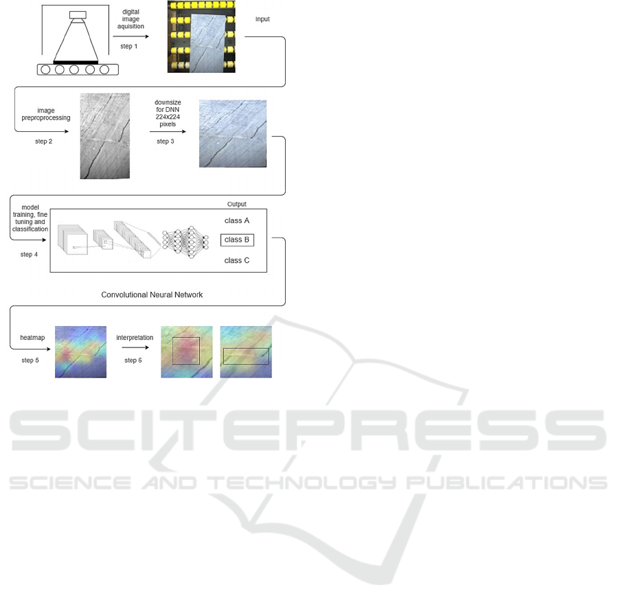
Figure 2: Pipeline of the methodology applied. Step 4 does

not depict a specific CNN. The example tile is classified as

class B.

2.2.1 Digital Image Acquisition

The original RGB digital images, from which the

dataset was compiled, were acquired by a device

consisting of a mechanical roller table, a digital

camera and a lighting setup. The roller table was fed

manually with the labelled marble tiles which were

photographed on the move by a MV_CA050-

10GM/GC digital camera equipped with a MVL-

MF0824M-5MP lens at a 90 cm distance. L.E.D.

arrays were used as a light source inside a diffusion

box.

2.2.2 Dataset Preprocessing

In order to feed the CNNs under examination, the

original RGB digital images, had to be preprocessed.

In the second step (Figure 2), noise from the

surrounding environment was removed, the tile was

extracted and the image was downsized. This was

achieved by converting the color space from RGB to

HSV followed by a Gaussian blur. Next, a threshold

was applied using a specific range of values followed

by the application of a contour detection algorithm

filtering out the vertical and horizontal lines. The

resulting four lines were used to determine the

corners of the rectangle tile. Finally, a perspective

transform was applied to align and to resize the tiles

to a 400x700 pixel vector.

CNNs have their own specific requirements for

the size of the inputs that they can handle. Therefore

the digital images had to be downsized to meet these

specifications. This was done in step 3 where the

preprocessed images were downsized to 224x224

pixels.

2.2.3 Convolutional Neural Networks

CNNs are essentially deep neural networks (DNNs)

specially developed for image classification. The

extensive use of DNNs in real world problems was

delayed for many years because high computational

power needed was not available. The progress in

computer hardware and especially in Graphical

Process Units (GPUs) of the recent years allowed the

usage of complex DNNs for numerous real world

problems encountered in the industry. In step 4 of the

proposed methodology, 15 pretrained CNNs using

the ImageNet database, available from the Keras

library (Chollet, 2015), were used to build the models

using the dataset of the 489 digital images of the

dolomite tiles. The pretrained models based on 15

CNNs were used, namely, DenseNet121 (DN121),

DenseNet169 (DN169), DenseNet201 (DN201)

(Huang et al., 2018)., InceptionResNetV2 (IRNV2)

(Szegedy et al., 2016), MobileNet (MN) (Howard et

al., 2017), MobileNetV2 (MNV2) (Sandler et al.,

2019), ResNet101 (RN101), ResNet152 (RN152),

ResNet50 (RN50), (He et al., 2015), ResNet101V2

(RN101V2), ResNet152V2 (RN152V2),

ResNet50V2 (RN50V2), VGG16, VGG19

(Simonyan & Zisserman, 2015) and Xception (XC)

(Chollet, 2017).

These aforementioned pretrained models were

fine-tuned applying the following modifications:

1. The original output layer of the NN was removed.

2. The model’s weights were frozen.

3. A Global AveragePooling2D was added, followed

by a Dropout layer with a 20% frequency rate to avoid

overfitting.

4. A Dense output layer using the softmax activation

function for the three quality classes was added

5. The output layer was trained with the training and

validation set of the current fold

6. The weights for only a part of the network’s layers

were unfrozen.

7. The unfrozen weights were trained again, with the

training and validation sets

It should be noted that the Adam optimizer was used

with a learning rate of 1e-5 and the categorical cross-

entropy function as the loss. Moreover, the backbone

Interpretable Deep Learning for Marble Tiles Sorting

103

of all the models was kept the same, without any

changes to the model itself, keeping the original input

shape of three channel images with a size of 224x224.

Additionally, the modifications 6 and 7 are part of the

fine-tuning of the transfer learning. These

modifications were applied in order to find the

number of trained layers that yielded the best

performance for the model. Moreover, the fine-tuning

was done for each additional quarter of the network’s

layers, meaning that we tested the network’s

performance by training 25% of the layers, 50%, 75%

and 100%. All models were trained with default

parameters and the number of layers used are

summarized in Table 1.

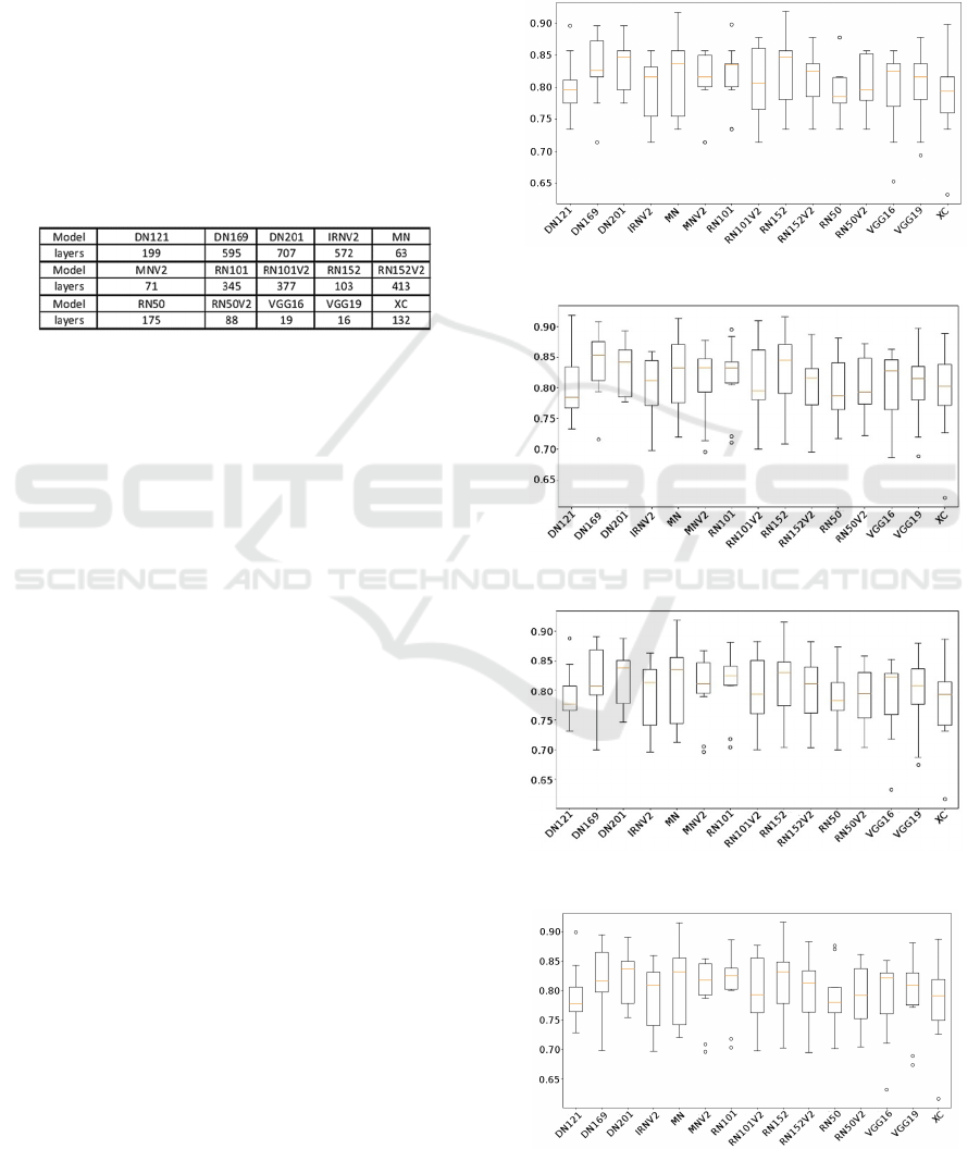
Table 1: Layers used to train each model.

A 10-fold cross validation technique was applied

for the evaluation of the CNNs, which were trained

for 50 epochs. The dataset was split initially to 90%

for training and 10% for testing, where the training

set was split again by 90% for training and 10% for

validation. The python programing language was

used to implement the code by using the Tensorflow

library (Abadi et al., 2015), for training the models,

and the machine learning library sklearn (Pedregosa

et al., 2018) for the evaluation. For the evaluation of

the models’ performance, the following metrics were

used: accuracy, precision, recall and f1-score.

2.2.4 Gradient-weighted Class Activation

Mapping

Until recently, Neural Networks were handled as

black boxes. The results from classification and

regression tasks were impossible to interpret.

Gradient-weighted Class Activation Mapping (Grad-

CAM) (Selvaraju et al., 2017) is an algorithm, which

outputs heatmaps of the images used for the training

of the CNNs. Heatmaps highlight, using colors, the

areas where the model is focusing on for extracting

the decisions, thus allowing the interpretation of the

results. Warm colors indicate important, whereas

colder colors indicate less important areas for the

model’s decisions. Areas not marked by any color

were not taken into account during the prediction

process. In the fifth step of this study, Grad-CAM is

applied for the interpretation of the results. In the

sixth step, the heatmaps’ output was interpreted in

order to validate the classification’s reliability

3 EXPERIMENTS

3.1 Results and Metrics

An overview of each metric versus the fine-tuned

model used can be examined in the boxplots of

Figure 3: Accuracy for the 15 CNNs.

Figure 4: Precision for the 15 CNNs.

Figure 5: Recall for the 15 CNNs.

Figure 6: F1 for the 15 CNNs.

DeLTA 2021 - 2nd International Conference on Deep Learning Theory and Applications

104

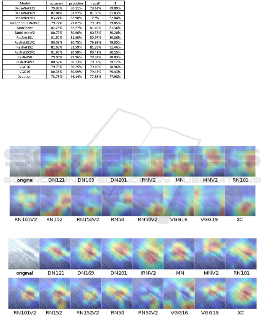
Figures 3-6. Each model’s metrics are summarized in

Table 2.

Table 2: Results of the experiments.

DN201 had the best overall performance: accuracy

=83.24%, precision=82.98, recall=82.00% and f1-

score=82.04%. DN169 achieved better precision with

a value of 83.97%, almost 1% better than the DN201,

but had an outlier. XC performed worst with

accuracy=78.73%, precision=79.14, recall = 77.88%

and f1-score = 77.98%. The boxplots show that the

DN201 is the most robust as it has the highest median

for all metrics excluding the precision. Also the

dispersion is comparable low. Other models like

MNV2 and RN101 have a lower dispersion but

outliers are present. All models have many outliers

except DN201, IRNV2, MN, RN101V2, RN152,

RN152V2 and RN50V2.

3.2 Interpretation of the Heatmaps

Heatmaps of all models, classifying successfully

three different sample tiles belonging to class A, B

and C are depicted in Figure 7, 8 and 9 respectively.

As it can be observed each model is not focusing on

the exact same area in order to classify each tile.

This confirms that each CNN is working in a

different way.

The probability of the correct classifications is

>99% in all than five cases: RN101V2 classified

sample 1 to class A (Figure 7) with a probability of

93.7%. DN121 classified sample 2 to class B (Figure

8) with a probability of 80.32%. MN, RN101 and

RN50 classified sample 3 to class C (Figure 9) with a

probability of 97.44%, 98.9% and 74.31%

respectively.

Figure 7: Heatmaps for the same marble tile (sample 1) successfully classified by all CNNs as class A.

Figure 8: Heatmaps for the same marble tile (sample 2) successfully classified by all CNNs as class B.

Interpretable Deep Learning for Marble Tiles Sorting

105

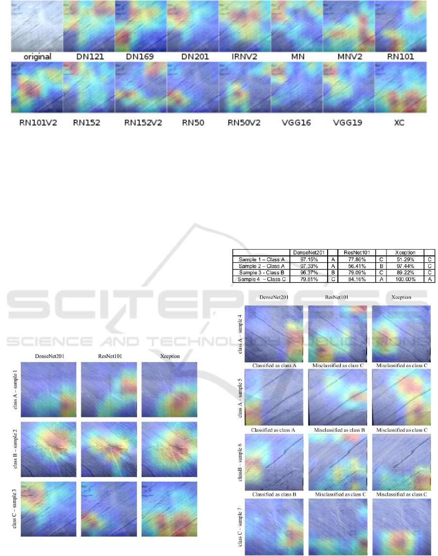
Figure 9: Heatmaps for the same marble tile (sample 3) successfully classified by all CNNs as class C.

By comparing the heatmaps (Figure 10) of the three

models representing the best (DN201, f1=82.04%),

the mean (RN101, f1=80.86%) and the worst (XC,

f1=77.98%) f1-score, the following qualitative

interpretation for the classification can be made: In

sample 1, DN201, RN101 and XC successfully

spotted the areas with alternating dark and light

colored lineation, which define class A. The best

classification metrics of DN201 can be attributed to

that it is not focusing on a specific structure of the tile

but rather draws conclusions from the whole tile in

class A. In sample 2, light colored intruding veins and

intersecting cracks were focused on, which define

class B. In sample 3, DN201 focused on the dark

inclusions, which characterizes class C. RN101 and

XC only focus partially (light blue color) on these

areas leading to lower metrics.

Figure 10: Heatmaps of the three representative CNNs,

correctly classifying three different marble tiles (sample 1-3).

In Figure 11 the heatmaps of DN201, RN101 and XC

are compared on tiles that were not successfully

classified by all models. In this comparison, the first

column represents the heatmaps of the DN201, which

successfully classified the samples, whereas the

second and the third column shows the heatmaps of

the models, RN101 and XC, which misclassified the

same samples. Table 3 lists the probability of each

classification

Table 3: Model’s classifying probability of samples.

Figure 11: Heatmaps of the three representative CNNs

classifying four different marble tiles (samples 4-7) with

correct and incorrect classification results.

DeLTA 2021 - 2nd International Conference on Deep Learning Theory and Applications

106

Sample 1 was correctly classified by DN201 to class

A with a probability of 97.15% by focusing on a

broader area where the alternating dark and light

colored lines are present. RN101 and XC incorrectly

classified the samples to class C with a lower

probability, 78.86% and 51.29% respectively,

focusing on discreet areas of dark lines and

misinterpreting them as spots.

Sample 2 was classified successfully as class A by

DN201 with a probability of 97.33%. RN101

incorrectly classified the sample as class B with a

probability of 56.41%, focusing on the light colored

intruding veins and XC classified it incorrectly as

class C, with a probability of 97.44%, by focusing on

the dark colored intruding veins.

Sample 3 was classified correctly as class B by

DN201 with a probability of 96.37%. RN101 and XC

models classified incorrectly the sample as class C by

focusing on the dark lines misinterpreting them as

dark spots with probabilities 79.09% and 89.22%

respectively.

Sample 4 was classified correctly as class C by

DN201 with a probability of 79.81%. Both RN101

and XC incorrectly classifies sample 4 as class A with

a probability of 84.16% and 100% by failing to focus

on the dark spots.

4 DISCUSSION

This paper tested the effectiveness of using pretrained

CNNs in order to classify natural dolomite rock tiles.

The results showed that this type of NN performs

better than conventional classifiers like Support

Vector Machine (SVM) (Cortes & Vapnik, 1995), K-

Nearest Neighbors (KNN) (Altman, 1992), Random

Forest (RF) (Breiman, 2001), Multilayer Perceptron

(MLP) (Popescu et al., 2009), Logistic Regressor

(Webb et al., 2011), Stochastic Gradient Descent

Classifier (SGD) (Ruder, 2017) and XGBoost

Classifier (XGB) (Chen & Guestrin, 2016) when

trained to discriminate dolomite tiles based on their

texture (Sidiropoulos et al., 2020).

Model DN201, using 707 layers, performed with

f1-score 82.04% trained with RGB images, whereas

the the XGBoost classifier trained by XCS-LBP

texture descriptors, achieved a performance of f1-

score 65.06% (Sidiropoulos et al., 2020).

By using Grad-CAM, it was possible to track the

areas on the surface of the tiles, which the model

focused on, in order to classify the tiles. This added

reliability to the results. The model build, focused on

the alternating light and dark colored banding for

identifying class A. Class B was recognized by the

model focusing on the light colored veins cutting the

banding in different angles. Class C was classified by

focusing on the dark spots.

In the next step of this research the best

performing model (DN201) will be reevaluated using

an augmented dataset using new techniques such as

MixUp (Zhang et al., 2018) and CutMix (Yun et al.,

2019). Furthermore the possibility of using a

combination of the CNNs studied in this paper to

compile an ensemble (Zhou, 2009) will be studied.

In the final stage of this project the resulting

model will be integrated into an automation system at

the facilities of Intermek Industrial & Trading Ltd.

This integration will permit the real-time

performance analysis of the proposed tiles sorting

model under industrial conditions.

ACKNOWLEDGEMENTS

This research has been co-financed by the European

Union and Greek national funds through the

Operational Program Competitiveness, Entre-

preneurship and Innovation, under the call

RESEARCH – CREATE – INNOVATE (project

code: T1EDK-00706).

REFERENCES

Abadi, M., Agarwal, A., & Barham, P. (2015). TensorFlow:

Large-Scale Machine Learning on Heterogeneous

Distributed Systems.

Altman, N. S. (1992). An Introduction to Kernel and

Nearest-Neighbor Nonparametric Regression. The

American Statistician, 46(3), 175–185. https://doi.org/

10.1080/00031305.1992.10475879

Breiman, L. (2001). Random Forests. Machine Learning,

45(1), 5–32. https://doi.org/10.1023/A: 1010933404324

Chen, T., & Guestrin, C. (2016). XGBoost: A Scalable Tree

Boosting System. Proceedings of the 22nd ACM

SIGKDD International Conference on Knowledge

Discovery and Data Mining, 785–794. https://doi.org/

10.1145/2939672.2939785

Chollet, F. (2015). Keras. GitHub Repository. https://

github.com/fchollet/keras

Chollet, F. (2017). Xception: Deep Learning with

Depthwise Separable Convolutions. ArXiv:1610.02357

[Cs]. http://arxiv.org/abs/1610. 02357

Cortes, C., & Vapnik, V. (1995). Support-vector networks.

Machine Learning, 20(3), 273–297. https://doi.org/

10.1007/BF00994018

Ferreira, A., & Giraldi, G. (2017). Convolutional Neural

Network approaches to granite tiles classification.

Expert Systems with Applications, 84, 1–11.

https://doi.org/10.1016/j.eswa.2017.04.053

Interpretable Deep Learning for Marble Tiles Sorting

107

He, K., Zhang, X., Ren, S., & Sun, J. (2015). Deep Residual

Learning for Image Recognition. ArXiv:1512.03385

[Cs]. http://arxiv.org/abs/1512. 03385

Hernandez, V. G., Perez, P. C., Perez, L. G. G., Balibrea, L.

M. T., & Puyosa Pina, H. (1995). Traditional and neural

networks algorithms: Applications to the inspection of

marble slab. 1995 IEEE International Conference on

Systems, Man and Cybernetics. Intelligent Systems for

the 21st Century, 5, 3960–3965. https://doi.org/10.

1109/ICSMC.1995. 538408

Howard, A. G., Zhu, M., Chen, B., Kalenichenko, D.,

Wang, W., Weyand, T., Andreetto, M., & Adam, H.

(2017). MobileNets: Efficient Convolutional Neural

Networks for Mobile Vision Applications.

ArXiv:1704.04861 [Cs]. http://arxiv.org/abs/1704.

04861

Huang, G., Liu, Z., van der Maaten, L., & Weinberger, K.

Q. (2018). Densely Connected Convolutional

Networks. ArXiv:1608.06993 [Cs]. http://arxiv.org/

abs/1608.06993

Laskaridis, K., Patronis, M., Papatrechas, C., Xirokostas,

N., & Flippou, S. (2015). Directory of Greek

Ornamental & Structural Stones. Hellenic Survey of

Geology & Mineral Exploration.

Liu, X., Wang, H., Jing, H., Shao, A., & Wang, L. (2020).

Research on Intelligent Identification of Rock Types

Based on Faster R-CNN Method. IEEE Access, 8,

21804–21812. https://doi.org/10.1109/ACCESS. 2020.

2968515

Lopez, M., Martinez, J., Matia, J. M., Taboada, J., & Vilan,

J. A. (2010). Functional classification of ornamental

stone using machine learning techniques. Journal of

Computational and Applied Mathematics, 234, 1338–

1345. https://doi.org/10.1016/j.cam.2010. 01.054

Martínez-Alajarín, J., Luis-Delgado, Jose. D., & Tomas-

Balibrea Luis M. (2005). Automatic System for

Quality-Based Classification of Marble Textures. IEEE

Transactions on Systems, Man, and Cybernetics—Part

C: Applications and Reviews, 35(5). https://doi.org/

10.1109/TSMCC.2005.843236

Martínez-Cabeza-de-Vaca-Alajarín, J., & Tomás-Balibrea,

L. (1999). Marble slabs quality classification system

using texture recognition and neural networks

methodology. Undefined. /paper/Marble-slabs-quality-

classification-system-using-Mart%C3%ADnez-Cabez

a-de-Vaca-Alajar%C3%ADn-Tom%C3%A1s-Balibre

a/371b 2875a024c6b58d97abb6801f202e219e326d

Pedregosa, F., Varoquaux, G., Gramfort, A., Michel, V.,

Thirion, B., Grisel, O., Blondel, M., Müller, A.,

Nothman, J., Louppe, G., Prettenhofer, P., Weiss, R.,

Dubourg, V., Vanderplas, J., Passos, A., Cournapeau,

D., Brucher, M., Perrot, M., & Duchesnay, É. (2018).

Scikit-learn: Machine Learning in Python.

ArXiv:1201.0490 [Cs]. http://arxiv.org/abs/1201.0490

Popescu, M.-C., Balas, V. E., Perescu-Popescu, L., &

Mastorakis, N. (2009). Multilayer Perceptron and

Neural Networks. WSEAS Trans. Cir. and Sys., 8(7),

579–588.

Ruder, S. (2017). An overview of gradient descent

optimization algorithms. ArXiv:1609.04747 [Cs].

http://arxiv.org/abs/1609.04747

Sandler, M., Howard, A., Zhu, M., Zhmoginov, A., & Chen,

L.-C. (2019). MobileNetV2: Inverted Residuals and

Linear Bottlenecks. ArXiv:1801.04381 [Cs]. http://ar

xiv.org/abs/1801.04381

Selvaraju, R. R., Cogswell, M., Das, A., Vedantam, R.,

Parikh, D., & Batra, D. (2017). Grad-CAM: Visual

Explanations from Deep Networks via Gradient-Based

Localization. 2017 IEEE International Conference on

Computer Vision (ICCV), 618–626. https://doi.org/

10.1109/ICCV. 2017.74

Sidiropoulos, G. K., Ouzounis, A. G., Papakostas, G. A.,

Sarafis, I. T., Stamkos, A., & Solakis, G. (2021).

Texture Analysis for Machine Learning Based Marble

Tiles Sorting. 2021 IEEE 11th Annual Computing and

Communication Workshop and Conference (CCWC),

2021, pp. 0045-0051, doi: 10.1109/CCWC51732.2021.

9376086.

Simonyan, K., & Zisserman, A. (2015). Very Deep

Convolutional Networks for Large-Scale Image

Recognition. ArXiv:1409.1556 [Cs]. http://arxiv.org/

abs/1409.1556

Solakis. (n.d.). Retrieved January 6, 2021, from https://

www.solakismarble.com/

Szegedy, C., Ioffe, S., Vanhoucke, V., & Alemi, A. (2016).

Inception-v4, Inception-ResNet and the Impact of

Residual Connections on Learning. ArXiv:1602.07261

[Cs]. http://arxiv.org/abs/1602. 07261

Webb, G. I., Sammut, C., Perlich, C., Horváth, T., Wrobel,

S., Korb, K. B., Noble, W. S., Leslie, C., Lagoudakis,

M. G., Quadrianto, N., Buntine, W. L., Quadrianto, N.,

Buntine, W. L., Getoor, L., Namata, G., Getoor, L.,

Han, X. J., Jiawei, Ting, J.-A., Vijayakumar, S., …

Raedt, L. D. (2011). Logistic Regression. In C. Sammut

& G. I. Webb (Eds.), Encyclopedia of Machine

Learning (pp. 631–631). Springer US.

https://doi.org/10.1007/978-0-387-30164-8_493

Yun, S., Han, D., Oh, S. J., Chun, S., Choe, J., & Yoo, Y.

(2019). CutMix: Regularization Strategy to Train

Strong Classifiers with Localizable Features.

ArXiv:1905.04899[Cs]. http://arxiv.org/abs/1905. 04899

Zhang, H., Cisse, M., Dauphin, Y. N., & Lopez-Paz, D.

(2018). mixup: Beyond Empirical Risk Minimization.

ArXiv:1710.09412 [Cs, Stat]. http://arxiv.org/abs/1710.

09412

Zhou, Z.-H. (2009). Ensemble Learning. In S. Z. Li & A.

Jain (Eds.), Encyclopedia of Biometrics (pp. 270–273).

Springer US. https://doi.org/10.1007/978-0-387-

73003-5_293

DeLTA 2021 - 2nd International Conference on Deep Learning Theory and Applications

108