Marine Vessel Tracking using a Monocular Camera
Tobias Jacob
a
, Raffaele Galliera
b
, Muddasar Ali
c
and Sikha Bagui
d
Department of Computer Science, University of West Florida, Pensacola, Florida, U.S.A.
Keywords:
Camera Calibration, Monocular Object Tracking, Object Detection, Error Prediction, Edge-ml, Distance
Estimation, YoloV5, Kalman Filters.
Abstract:
In this paper, a new technique for camera calibration using only GPS data is presented. A new way of tracking
objects that move on a plane in a video is achieved by using the location and size of the bounding box to
estimate the distance, achieving an average prediction error of 5.55m per 100m distance from the camera. This
solution can be run in real-time at the edge, achieving efficient inference in a low-powered IoT environment,
while being also able to track multiple different vessels.
1 INTRODUCTION
Ship avoidance systems are typically based on radio
signals. In this paper, a new technique for camera
calibration using only GPS data is presented. To get
a better position estimate from an object detector, the
property that ships move on a plane is utilized. Also,
a new way of tracking objects that move on a plane in
a video is achieved by using the location and size of
the bounding box to estimate the distance.
This approach has many possible use cases in edge
computing. This includes tracking airplanes in air-
ports, ships in harbours, cars in parking lots or hu-
mans in shopping malls. It also demonstrates how to
efficiently track one specific object from other similar
instances of that object. This can play an important
role in traffic systems. For example, it is possible to
keep track of free spaces in a parking lot. This infor-
mation could be utilized in various IoT applications
helping citizens to find a free parking space. Another
use case is smarter traffic lights, which could use a
camera to react to oncoming traffic quicker. For this,
all that is needed for camera calibration and train-
ing or evaluating the object detector is 33 minutes of
videos and ground truth GPS positions or something
comparable. The methods utilized in this paper are
fast enough to be deployed on inexpensive edge com-
puting devices that can be mass-produced.
a
https://orcid.org/0000-0002-8530-258X
b
https://orcid.org/0000-0001-7777-3835
c
https://orcid.org/0000-0002-6044-9892
d
https://orcid.org/0000-0002-1886-4582
2 RELATED WORK
A rich background of GPS camera calibration papers
are available(e.g. (Liu et al., 2010)), but to date, none
of these works use just GPS data to determine lens
distortion of a single camera. The novelty of this pa-
per is that it introduces an algorithm that relies on data
from a single camera without any a-priori informa-
tion about the camera parameters. Research has also
been done for monocular position tracking with a cal-
ibrated camera. (Ali and Hussein, 2016) used a car-
mounted front-facing calibrated camera and Hough
Transformations (Duda and Hart, 1972) to extract the
distance to other cars. They achieve an average lat-
eral error of 9.71%. The error is measured as dif-
ference between prediction and ground truth in me-
ters per 100 meters distance from the camera. (Dhall,
2018) presents a combination between YoloV2 and
a keypoint detector to achieve an average error of
6.25%. (Hu et al., 2019) uses Faster R-CNN for object
detection and an additional network for 3D Box esti-
mation, reaching an average position error of 7.4%.
Monocular position estimation is closely related to
depth estimation. Recent methods achieved between
7.1% and 21.5% accuracy (Bhoi, 2019).
Some solutions have been proposed for Un-
manned Aerial Vehicles (UAVs). (Sanyal et al., 2020)
suggests an approach to detect and estimate the loca-
tion of an object in an environment where the UAV
operates with a single monocular camera using its
GPS position. Given the home position, the GPS lo-
cation of the UAV, and the image taken from the cam-
era, the authors have developed a method to estimate
the depth of an object in the image after detecting it
Jacob, T., Galliera, R., Ali, M. and Bagui, S.
Marine Vessel Tracking using a Monocular Camera.
DOI: 10.5220/0010516000170028
In Proceedings of the 2nd International Conference on Deep Learning Theory and Applications (DeLTA 2021), pages 17-28
ISBN: 978-989-758-526-5
Copyright
c
 2021 by SCITEPRESS – Science and Technology Publications, Lda. All rights reserved
17

using Yolo. (Leira et al., 2017) Developed a solution
for UAVs with computational power and an onboard
camera to detect, recognize, and track multiple ob-
jects in a maritime environment. The system was able
to automatically detect and track the position and the
velocity of a boat with an accuracy of 5-15 meters, be-
ing at a height of 400 meters. Furthermore, the track-
ing could be done even when a boat was outside the
FOV (field of view) for extended periods of time.
In summary, several applications have been imple-
mented for detection and tracking of objects present
in a view of the camera, but not much work has been
done on developing solutions that could run at the
edge, leveraging low-powered IoT commercial off-
the-shelf devices, which this work presents.
3 METHODS
The data consists of videos, a time series of GPS po-
sitions of the vessel and the GPS position of the cam-
era. First the relation between the world position of
the vessel and the on-screen position is determined.
Then, an object detector is trained to track the vessel
on the image. Post-processing is applied to increase
stability and precision.
3.1 Converting World/ Screen
Let (ϕ,λ) be the latitude and longitude in arc measure,
respectively, of the ship, and similarly (ϕ
0
,λ
0
) be the
position of the camera. The camera is at the origin
at the world coordinate system, while the ship is at
(x
w
,y
w
). The distance in meters can be obtained with
an equi-rectangular projection (Snyder, 1987):
x
w
= r(λ − λ
0
)cosϕ
0
, (1)
y
w
= r(ϕ − ϕ
0
), (2)
with r = 6371 km being the earth radius (Moritz,
2000). The ship is always at sea level, so z
w
= 0 can
be omitted. The following homo-graphic equation has
to be solved:
z
p


x
p
y
p
1


= H


x
w
y
w
1


. (3)
(x
p
,y
p
) are the projected coordinates. z
p
is the dis-
tance from the camera to the vessel. H is a matrix that
projects the world coordinates to the screen. The cam-
era has significant lens distortion. This means that the
final coordinate (x , y) of the ship on screen and the
projected coordinates (x
p
,y
p
) have the relationship:
x
p
= x
s
+ (x
s
− x
c
)(1 + K
1
r
2
), (4)
y
p
= y
s
+ (y
s
− y
c
)(1 + K
1
r
2
), (5)
where (x
c
,y
c
) is the center of the image and r
2
the
distance from the center of the image.
r
2
= (x
s
− x
c
)
2
+ (y
s
− y
c
)
2
. (6)
K
1
and H are parameters that have to be learned.
We created a dataset containing 11 hand-labeled pairs
of screen positions (x
s,lab
,y
s,lab
) and GPS positions
(λ,ϕ). The GPS data was reconstructed from the
video and frame index using a linear interpolation of
the timestamps provided and a linear interpolation of
the GPS data for that timeframe. The least squares so-
lution for equation 3 for H can be easily computed. K
1
introduces a non-linearity, hence it was brute-forced.
The result is shown in figure 5b. Different values
for K
1
were used for calculating (x
p,lab
,y
p,lab
) from
(x
s,lab
,y
s,lab
) and solving equation 3 for H, and mea-
suring the MSE between the estimated screen posi-
tion (x
p
,y
p
) and the hand-labeled screen position for
all labeled points i.
Loss =
∑
i
(x
p,i
− x
p,lab,i
)
2
+ (y
p,i
− y
p,lab,i
)
2
. (7)
3.2 Object Detection
The recent advancements of Deep Learning-based ob-
ject detection models were state-of-art in achieving
improvements in terms of both inference time and re-
liability of the predictions (Jiao et al., 2019). Dealing
with the hardware constraints present in edge devices
brings additional attention to the need of smaller mod-
els performing fast inference, while keeping the accu-
racy of predictions as high as possible. We found two
architectures and implementations, YoloV5 (Jocher
et al., 2020) and EfficientDet (Tan et al., 2020)
playing a key role in object detection model sce-
narios, offering different configurations in terms of
model sizes. We tested both models on a standard
NVIDIA Jetson Nano Developer Kit, a small, com-
mercial off-the-shelf device for AI embedded appli-
cations, equipped with 4GB of LPDDR4 RAM, 128-
core Maxwell GPU and a Quad-core ARM A57 CPU.
As presented in table 1, YoloV5s was found to
be the best solution for resource constrained de-
vices like the NVIDIA Jetson Nano, in terms of
trade-off between mAP (mean Average Precision)
and FPS (Frames per Second) processed, when us-
ing 320x320px images. Once camera calibration and
H and K
1
are known, they can be used to predict the
Bounding Box (c
x
,c
y
,s
x
,s
y
) of the vessel. Let (c
x
,c
y
)
be the location of the ship. The dimensions of the
DeLTA 2021 - 2nd International Conference on Deep Learning Theory and Applications
18

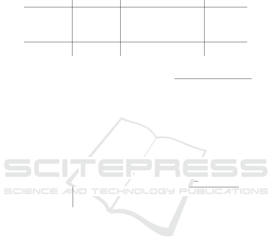
Table 1: Comparison of different YoloV5 and EfficientDet configurations, with mean Average Precision evaluated on a
NVIDIA JetsonNano on COCO (Lin et al., 2015) 2017 validation dataset and FPS performance reported on a 720p video.
Models are sorted by type (Yolo, EfficientDet), size of the model, and image resolution adopted.
Model Image resolution mAP (mean Average Precision) Processed FPS
YoloV5x 416x416px 0.451 1.25
YoloV5l 416x416px 0.328 2.48
YoloV5m 416x416px 0.402 3.11
YoloV5s 416x416px 0.333 8.70
YoloV5s 320x320px 0.299 10.75
EfficientDet(D0) 256x256px 0.336 7
EfficientDet(D1) 256x256px 0.394 5
bounding box (s
x
,s
y
) are set on half image resolution
to:
s
x
= (1500/z
p
+ 25) , (8)
s
y
= (850/z
p
+ 25) . (9)
z
p
is the distance from the vessel to the camera in
project space, as obtained by equation 3. The scale
factors were empirically chosen to include the ves-
sel and have a minimum size of 25. An example is
shown in figure 1. To not process unnecessary data,
the image is scaled down by 2 and cropped to the up-
per (640,192) pixels. Besides the hyper-parameters
shown in table 2, the default hyper-parameters of
YoloV5s were used.
Table 2: Training hyper-parameters that differ from the de-
fault values.
Epochs 20
Batch size 16
Image size 352
3.3 Post Processing
Outputs of the networks tend to be noisy. They might
detect no ship, a slightly off position, multiple bound-
ing boxes for the same ship, or multiple ships.
First, the trajectories for every ship have to be ob-
tained. Each trajectory uses a Kalman filter (Kalman,
1960) to predict the location in the next frame. All
detected ships in the next frame are accounted to the
closest trajectory if they are within 80 pixels of the ra-
dius. Each trajectory is updated with the closest point
that was accounted to it. A trajectory is finished if
it is not updated for more than 10 frames. In case
no trajectory is found for a detection, it is considered
new. Out of those trajectories, the correct one has to
be found. The trajectory score is defined as:
score = c
0.8l
logl . (10)
c is the sorted confidence values that YoloV5s issued
to the trajectory positions with l being the trajectory
length for all data points i of the trajectory.
l =
l−1
∑
i=1
q
(x
w,i
− x
w,i+1
)
2
+ (y
w,i
− y
w,i+1
)
2
. (11)
c
0.8l
represents the 80th percentile of c. It was as-
sumed that the trajectory with the highest score was
the vessel we were looking for. When the trajectory
got cut in the middle, other trajectories were found
that would be pre- or appended to the current trajec-
tory by looking at the timestamps.
x
p,Yolo
and y
p,Yolo
can be obtained directly from
the object detector and camera calibration. The
bounding box size is used as an additional indicator
for distance z
p
and vertical position y
p
. z
p,s
x
and z
p,s
y
can be obtained from equation 8.
y
p
=
±
1
z
p
− H
−1
2,0
x
p
− H
−1
2,0
H
−1
2,1
. (12)
The different predictors are shown in figure 2. The fi-
nal estimate of the y position is the weighted average:
y
p
= 0.5y
Yol o
+ 0.25y
p,s
x
+ 0.25y
p,s
y
. (13)
The parameters were empirically chosen since the po-
sition based predictor is less noisy than the bound-
ing box size based predictors, as shown in figure 2.
Finally, a Kalman filter is used to smooth the com-
posed trajectory and estimate missing values. Points
that have a vertical difference of more than 5 pixels
to the smoothed trajectory are considered outliers and
masked out. Then the algorithm runs again, 5 times
in total. A masked out point may become unmasked
if the smoothed trajectory moved closer to it. The
effect is shown in figure 3. Then, the GPS coordi-
nate of the vessel can be obtained by reversing the
equations in section 3.1. In case the point is above
the horizon (z
p
has wrong sign), or very far, it is ex-
cluded. Missing data points may be obtained using a
cubic interpolation of the data. The output is clipped
to [−2000,2000] for safety.
All Kalman filters use the following state-
transition F
k
, observation R
k
, transition co-variance
Marine Vessel Tracking using a Monocular Camera
19

Q
k
and observation co-variance R
k
, with ∆ being the
time in seconds between frames:
F
k
=



1 1 0 0
0 1 0 0
0 0 1 1
0 0 0 1



, (14)
H
k
=

1 0 0 0
0 0 1 0

, (15)
Q
k
= diag(0,1∆
2
,0,1∆
2
), (16)
R
k
= diag(10
2
,10
2
). (17)
4 RESULTS
All methods were validated on the dataset of the “AI
tracks at sea” Challenge (Tall, 2020). This dataset
contained 11 videos, each 3 minutes in time, and
ground truth GPS positions for the ship.
4.1 Camera Parameters
The learner for inferring the camera parameters dis-
covered the following K1 and H values:
K
1
= −4.053 · 10
−7
, (18)
H ≈


4.41 · 10
2
3.79 · 10
2
−1.00 · 10
3
−2.17 · 10
2
−5.65 · 10
1
−5.48 · 10
2
−5.12 · 10
−1
−1.44 · 10
−1
1 · 10
0


.
(19)
The results are visualized in figure 4. The orange line
in figure 4a is characterized by the vanishing points of
the plane:
x
p,hor
H
−1
3,1
+ y
p,hor
H
−1
3,2
= −H
−1
3,3
. (20)
It matches the actual horizon within 5 pixels. The
difference between our hand-labeled points and the
project points is shown in figure b. The loss is visi-
ble as the mean squared error between the orange and
blue points, indicated by the green lines. The cam-
era orientation can also be obtained. With x
p,hor
= x
c
being in the middle of the image and y
p,hor
fulfilling
equation 20, the horizon point can be deprojected us-
ing:


x
w,hor
y
w,hor
0


= H
−1


x
p,hor
y
p,hor
1


. (21)
The heading of the camera is:
α = arctan
x
w,hor
y
w,hor
= 76.5
◦
. (22)
This allows for the adjustment of the orientation of
the camera by multiplying (x
w
,y
w
) with a 2D rotation
matrix.
4.2 Object Detection
14 videos that contained recorded camera imagery of
sea vessel traffic along with the recorded GPS track of
the vessel of interest were used for this work. The net-
work was trained on 6 Videos (7, 8, 9, 10, 11 and 12)
and 5 videos (13, 14, 15, 16, and 17) were used for
validation. Videos 18, 19 and 20 did not have GPS
data, so they could only be used for testing. For fi-
nal results, the network was trained for one additional
epoch on the training and validation dataset. The re-
sults shown in this paper are without training on the
validation set.
Two situations occurred depending on the train-
ing length. If YoloV5s was trained for 50 epochs, it
was able to distinguish the vessel from other ships like
sailboats and jetskis on the training data, but it per-
formed poorly on validation due to overfitting, which
started after epoch 20. After 20 training epochs,
YoloV5s not only detected the ship well, but also
other ships like sailboats and jetskis. Filtering the cor-
rect ship out of all the generated trajectories turned
out to be a major source of error.
4.3 Post Processing
YoloV5s infers a position that is 2 pixels (on half res-
olution) above the actual on-screen position needed.
Therefore, this was added as a fixed offset to the po-
sitions that the network inferred. This could be at-
tributed to the fact that the pre-trained YoloV5s used
a different center point on objects. The Kalman fil-
ters are able to remember the velocity of each ves-
sel. When two vessels cross each other, they can keep
track of both trajectories, as shown in figure 6. In
video 18 the model is able to interpolate the out-of-
screen position of the vessel with the information of
how the vessel left and reentered the frame.
The result of the final pipeline is shown in fig-
ure 7 and figure 8. The error for 4 out of 5 videos
is less than 20 m. The error is also proportional to
the distance. At a distance of 150 meters, if the ship
at (x
w
,y
w
) moves roughly 10m away from the cam-
era ((150,50) to (160,53)), this equates to a vertical
change of roughly 0.276 pixels on the half resolution
the network is working on. This approach is working
with a sub-pixel accuracy.
4.4 Performance
On the NVIDIA Jetson Nano used for testing, 5.31
FPS was reached for the whole pipeline. YoloV5s
took 72% of that time, while the other 28% can be
mostly attributed to video decoding. Considering that
DeLTA 2021 - 2nd International Conference on Deep Learning Theory and Applications
20

1 FPS is enough for the algorithm to produce a stable
output, this algorithm is easily capable of running in
real-time on low-powered embedded devices.
4.5 Validation
The main objective is to validate performance calcu-
lating the inference error of the model, which repre-
sents the distance in meters from the ground truth po-
sition against the distance in meters from the video
source. A correlation between these two factors
would be valuable for different reasons, starting from
the most obvious understanding of how the model is
performing to having the possibility of adding a pre-
diction of the error to the pipeline. The possibility of
making such a prediction is a great improvement of
the whole pipeline, both from a technical as well as
user-end perspective. Practically, along the predicted
position of the target vessel, the output will be en-
riched with the approximation of error.
This section explains how to perform the distance
estimation of the vessel from the camera. The dis-
tance of the predicted point from the ground truth will
also be presented, ending with a brief explanation of
possible error prediction methods. As mentioned in
the Object Detection section, the validation has been
performed on five different videos (videos 13, 14, 15,
16 and 17), for a total amount of 713 data points.
4.5.1 Distance Estimation
In order to calculate the distance from the camera and
the actual error from the predicted point, the Haver-
sine formula (M, 2010) is used. The formula calcu-
lates the shortest distance between two points on a
sphere using their latitude and longitude, and is ex-
pressed as follows:
d = 2r arcsin
r
sin
2
φ
2
− φ
1
2
+ cos φ
1
cosφ
2
sin
2
λ
2
− λ
1
2
(23)
r is the radius of the earth in meters, φ
1
,φ
2
is the
latitude of the two points, and λ1,λ2 is the longitude.
4.5.2 Considerations about the Validation Set
The distance from the camera of the target vessel is
approximately between 86 and 200 meters for 75% of
the data points, with peaks of 2500 meters. One of
the videos, however, represent a particular issue for
the validation process, as its frames show the vessel
from the back and at a close distance, a point of view
which is unique in this dataset. A possible solution
could consist of shrinking the testing set by including
the video in the training process. Although this work
aims at getting the best performance possible in terms
of inference and generalization with a limited amount
of data points, we found that the model is not able to
generalize to that level in this constrained scenario.
4.5.3 Validation Results
As shown in Figures 8 and 9, the error performed by
the model is below 20 meters for 80% of the valida-
tion data points, the only outlying points are the ones
belonging to Video 17, reaching important errors at
high distances. Some of these points represent the
model detecting another vessel, which was mislead-
ing these predictions. However, it can be noted that
the model is able to predict positions around 500 and
1000 meters with a small amount of error. Predic-
tions in the testing dataset have the highest density
well below 20 meters, even reaching a precision be-
low a single meter at the highest distances [Figures 8,
9]. It is now possible to use all the extrapolated infor-
mation to perform error prediction at the end of the
pipeline. The first stage of the work predicts the posi-
tion of the vessel performing on the validation set. Af-
ter that, the Haversine distance between both the pre-
dicted distance and ground truth, as well as the ground
truth and camera position, are computed. These two
parameters are used to feed the error prediction mod-
els and are respectively called prediction error and
distance from camera. The experimental results pre-
sented include the usage of classic Machine Learning
methods, Linear Regression and Support Vector Ma-
chine, applied to regression problems, that is, SVR, as
well as a Deep Learning approach.
The first concern is, once again, the dataset. A
plausible solution is to split the previous validation set
according to Videos, excluding video 17. By includ-
ing video 17, the predicted distance from the model
would only be uncontrolled noise to our dataset, with-
out adding any value to the scope. The training set is
now composed of 429 data points belonging to Videos
14, 15 and 16, while the testing set has 143 points
from Video 13. SVR adopts an approach similar to
Support Vector Machines as Large Margin Classifiers
(Cortes and Vapnik, 1995), with the usage of kernel
tricks (Aizerman et al., 1964) to create Nonlinear clas-
sifiers. The quality of the hyperplane is determined by
the points falling inside the decision boundary. The
results presented by Table 4 show that a simple net-
work, with only two hidden layers and trained for 5
epochs, is able to reach a Root Mean Squared Er-
ror between 4 and 5 meters, using a batch size of 32
data points. The Neural Network performance is also
shown by Figure 9. The SVR, using the Radial Ba-
sis Function kernel to approximate the nonlinear be-
Marine Vessel Tracking using a Monocular Camera
21

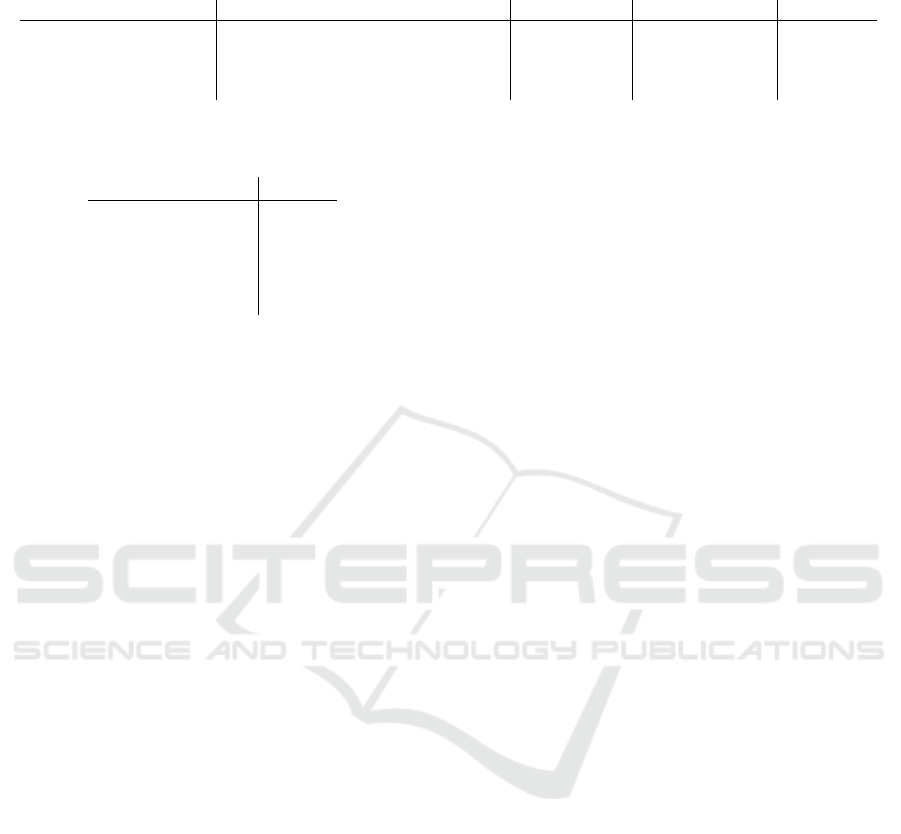
Table 3: Comparison of tracking accuracy with others. The average error is measured in meters per 100 meters distance.
Different cameras, angle of views, target objects, and image resolution make a direct comparison hard to value.
Paper Method Target Object Image resolution Avg. error
(Ali and Hussein, 2016) Hough Transform Cars 480x360 9.71%
(Hu et al., 2019) Faster R-CNN and 3D box prediction Cars 1392x512 7.40%
(Dhall, 2018) YoloV2 and keypoint prediction Cone Not stated 6.25%
Ours YoloV5s Vessel 640x360 5.55%
Table 4: The Root Mean Squared Error - RMSE - in meters
from the actual predicted point.
Method RMSE
DNN 4.95
Linear Regression 6.88
SVR(Linear) 6.96
SVR(Polynomial) 8.35
SVR(RBF) 6.04
haviour, was initially prone to overfitting, achieving
worse results then the Linear kernel on the testing set.
To overcome this undesirable situation, the allowed
margin error was increased in the training set. This al-
lowed to generalize better than the Linear Regression
and SVR models. The final linear regression learned
is:
˜e = 0.0555d . (24)
This means that the accuracy of the pipeline is 5.55m
per 100 m distance. More data points and further ex-
perimentation would, of course, strengthen the infer-
ence capabilities of these models. Error prediction
can play a significant role in the pipeline depending
on the use case where this methodology could be ap-
plied. In fact, external decision-making systems could
opt for a certain action, or verification, depending on
the detected distance of the object.
5 DISCUSSION AND FUTURE
WORK
The results in table 3 show that our model reaches
state-of-the-art precision when compared with other
methodologies. However, comparisons are imprecise,
because of many factors like the angle of view, reso-
lution, camera position or target object that could in-
fluence the result. Our approach efficiently exploits
GPS data with a fast and reliable inference for closer
distances, bringing great advantage in terms of possi-
ble useful insights, like a subsequent precise distance
estimation.
We can figure different applications in both small
and large scenarios. For example, tracking a car in
a parking lot, where the camera is close and the ac-
curacy proved to be high. A larger use-case might
be keeping track of traffic in a container ship port or
airport, where the camera is further away but the ob-
jects are larger, and in this way this approach main-
tains the same relative accuracy. This method could
also be easily extended for cases with z
w
6= 0, as long
as there is a clear mapping from (x
w
,y
w
) → z
w
and
(x
p
,y
p
) → z
p
.
As stated, the average error is 5.55m per 100m dis-
tance and the network is able to track the ship within a
sub-pixel resolution, which is crucial for distance re-
liability. The accuracy could be further improved by
using a steeper camera angle and more training data,
as well as the performance in terms of FPS improved
adopting TensorRT network definition APIs and 8-bit
inference(Migacz, 2017). A particular challenge for
the network is to learn to distinguish the vessel from
other ships like jet-skis or sailboats. This leads to the
problem that multiple ships may be detected. A style
detector, as presented in (Wojke et al., 2017), could be
used to differentiate between different ships. When
the object is moving quickly or the data point resolu-
tion is poor, the algorithm struggles with inferring the
trajectories. For ships, a data point every second is
recommended.
In edge cases, for example when the ship leaves
the frame, the whole pipeline is very sensitive to the
hyper-parameters chosen, for example, how long a
trajectory lasts without new positions. In more stan-
dard situations, when the ship is in a reasonable dis-
tance and well visible, the algorithm is stable and pre-
cise. Since our approach requires a single frame every
second, it can easily be run on resource constrained
devices at the edge achieving a low inference time,
while being able to track a specific vessel as well as
multiple different ones, depending on the needs and
training data available.
REFERENCES
Aizerman, M. A., Braverman, E. A., and Rozonoer, L.
(1964). Theoretical foundations of the potential func-
tion method in pattern recognition learning. Automa-
tion and Remote Control, 25:821–837.
Ali, A. A. and Hussein, H. A. (2016). Distance estima-
tion and vehicle position detection based on monoc-
ular camera. In 2016 Al-Sadeq International Confer-
ence on Multidisciplinary in IT and Communication
DeLTA 2021 - 2nd International Conference on Deep Learning Theory and Applications
22

Science and Applications (AIC-MITCSA), pages 1–4.
Bhoi, A. (2019). Monocular depth estimation: A survey.
Cortes, C. and Vapnik, V. (1995). Support vector networks.
Machine Learning, 20:273–297.
Dhall, A. (2018). Real-time 3d pose estimation with
a monocular camera using deep learning and ob-
ject priors on an autonomous racecar. CoRR,
abs/1809.10548.
Duda, R. O. and Hart, P. E. (1972). Use of the hough trans-
formation to detect lines and curves in pictures. Com-
mun. ACM, 15(1):11–15.
Hu, H.-N., Cai, Q.-Z., Wang, D., Lin, J., Sun, M.,
Kr
¨
ahenb
¨
uhl, P., Darrell, T., and Yu, F. (2019). Joint
monocular 3d vehicle detection and tracking.
Jiao, L., Zhang, F., Liu, F., Yang, S., Li, L., Feng, Z., and
Qu, R. (2019). A survey of deep learning-based object
detection. IEEE Access, 7:128837–128868.
Jocher, G., Stoken, A., Borovec, J., NanoCode012, Christo-
pherSTAN, Changyu, L., Laughing, tkianai, Hogan,
A., lorenzomammana, yxNONG, AlexWang1900, Di-
aconu, L., Marc, wanghaoyang0106, ml5ah, Doug,
Ingham, F., Frederik, Guilhen, Hatovix, Poznanski, J.,
Fang, J., Yu, L., changyu98, Wang, M., Gupta, N.,
Akhtar, O., PetrDvoracek, and Rai, P. (2020). ultra-
lytics/yolov5: v3.1 - Bug Fixes and Performance Im-
provements.
Kalman, R. E. (1960). A new approach to linear filtering
and prediction problems. Transactions of the ASME–
Journal of Basic Engineering, 82(Series D):35–45.
Leira, F. S., Helgesen, H. H., Johansen, T. A., and Fos-
sen, T. I. (2017). Object detection, recognition, and
tracking from uavs using a thermal camera. Journal
of Field Robotics.
Lin, T.-Y., Maire, M., Belongie, S., Bourdev, L., Girshick,
R., Hays, J., Perona, P., Ramanan, D., Zitnick, C. L.,
and Doll
´
ar, P. (2015). Microsoft coco: Common ob-
jects in context.
Liu, H., Wang, C., Lu, H., and Yang, W. (2010). Outdoor
camera calibration method for a gps camera based
surveillance system. In 2010 IEEE International Con-
ference on Industrial Technology, pages 263–267.
M, M. M. G. (2010). Landmark based shortest path detec-
tion by using a* and haversine formula. International
Journal on Recent and Innovation Trends in Comput-
ing and Communication, 6(7):98–101.
Migacz, S. (2017). 8-bit inference with tensorrt. GPU Tech-
nology Conference.
Moritz, H. (2000). Geodetic reference system 1980. Jour-
nal of Geodesy, 74(1):128–133.
Sanyal, S., Bhushan, S., and Sivayazi, K. (2020). Detection
and location estimation of object in unmanned aerial
vehicle using single camera and gps. In 2020 First In-
ternational Conference on Power, Control and Com-
puting Technologies (ICPC2T), pages 73–78.
Snyder, J. P. (1987). Map projections: A working manual.
Technical report, Washington, D.C.
Tall, M. H. (2020). Ai tracks at sea. https://www.challenge.
gov/challenge/AI-tracks-at-sea/.
Tan, M., Pang, R., and Le, Q. V. (2020). Efficientdet: Scal-
able and efficient object detection.
Wojke, N., Bewley, A., and Paulus, D. (2017). Simple on-
line and realtime tracking with a deep association met-
ric.
Marine Vessel Tracking using a Monocular Camera
23

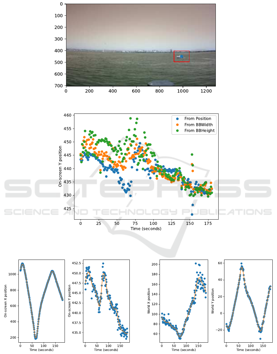
Figure 1: Example of bounding box size. It is empirically chosen to fit the boat.
Figure 2: The y
p
by the two bounding-box-size-based estimators as in equation 12 and the bounding-box-center-based pre-
dictor.
(a) Effect of the Kalman filter for smoothing the trajectory
in screen coordinates.
(b) Effect of the Kalman filter for smoothing the trajectory
in world coordinates.
Figure 3: The Kalman filters are a crucial step in obtaining a smooth trajectory, particularly for lateral movement.
DeLTA 2021 - 2nd International Conference on Deep Learning Theory and Applications
24

(a) Visualization of the learned camera parameters. The grid shows 10 meter squares, with 100 > x
w
> 10 and
100 > y
w
> 0. Note the effect of the lens distortion, and how the orange line matches the horizon. The blue
vanishing point is exactly east.
(b) The difference between our hand labeled points and the projected GPS coordinates.
Figure 4: Evaluation of the Camera Parameters.
Marine Vessel Tracking using a Monocular Camera
25

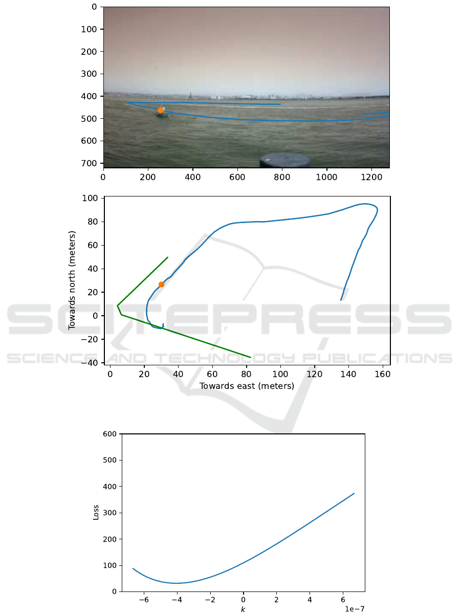
(a) An example of a GPS track mapped into the video. Note that the camera is facing eastwards and not perfectly
horizontal. The green lines indicate the rectangle x
s
∈ [0,1280], y
s
∈ [440,720].
(b) Brute force evaluation of the lens distortion parameter K
1
Figure 5: Evaluation of the Camera Parameters.
DeLTA 2021 - 2nd International Conference on Deep Learning Theory and Applications
26

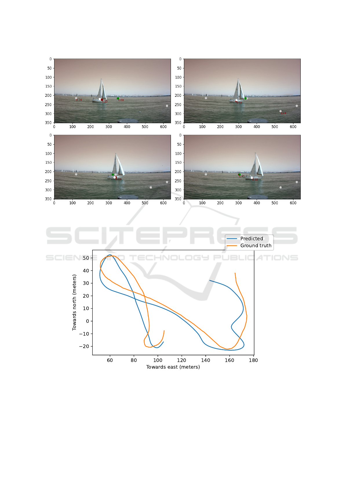
Figure 6: Green is the smoothed trajectory of the vessel. White/Grey is the trajectory of a ship in general (white when it got
detected in this frame, grey if it has not been detected in the current frame and position is guessed). Red are detected points
in the image. They may be obscured by the white points. When the vessel is behind the sailboat, the grey and green point
estimate the position.
Figure 7: Validation of the complete pipeline using Video 15. Showing the Ground Truth track of the vessel (orange line)
against the predicted one (blue line).
Marine Vessel Tracking using a Monocular Camera
27

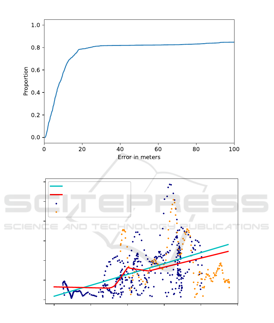
Figure 8: Distribution of the error in meters, output of our pipeline. 80% of the predictions have an error below 20 meters.
Linear Regression
Deep Neural Network
Target distance from camera
Error in meters
Training Data
Testing Data
0
0
50
100
150
200
250
5
10
15
20
25
30
Figure 9: Visualization of the error prediction performance on the error prediction validation set. The linear regression show
the average error is 5.55m per 100m distance from camera. The distance of the target vessel from the camera, against the error
in meters produced by the predictions is plotted, with the training data points in blue and validation in orange. The learned
regression from the Linear Regression modelling (light-blue) and the Deep Neural Network (red) is showed.
DeLTA 2021 - 2nd International Conference on Deep Learning Theory and Applications
28