An Evolutionary Calibration Approach for Touch Interface Filter Chains
Lukas Rosenbauer
1
, Johannes Maier
1
, Daniel Gerber
1
, Anthony Stein
2
and J
¨
org H
¨
ahner
3
1
BSH Hausger
¨
ate GmbH, Im Gewerbepark B35, Regensburg, Germany
2
Artificial Intelligence in Agricultural Engineering, University of Hohenheim, Garbenstr. 9, Stuttgart, Germany
3
Organic Computing Group, University of Augsburg, Am Technologiezentrum 8, Augsburg, Germany
Keywords:
Automation, Optimization, Bio-inspired Computation, Intelligent Computing, Genetic Algorithm,
Calibration, Signal Processing, Human Machine Interface.
Abstract:
Touch interfaces are human machine interface (HMI) that can be found in a wide range of products ranging
from mobile phones over cars to home appliances. Many of these HMIs measure digital signals which are
used to detect touch events. These signals are processed using filters in order to decide whether there is a
touch event or not. The filterchain must be functional even if the signal contains heavy noise. Thus a precise
calibration of the individual filters is necessary. We employ a genetic algorithm (GA) to choose the filter
parameters automatically. We evaluate our approach in a series of experiments which includes simulated as
well as real data. We additionally compare our GA with manually calibrated parameters and thereby show
the superiority of our method in terms of the accuracy of the calibration provided. A cost-intensive manual
calibration can thus be avoided.
1 INTRODUCTION
Evolutionary computation has led to advances in sev-
eral fields. Applications include the automated de-
sign of digital circuits (Ryan et al., 2020), material
fault detection (Margraf et al., 2017) and automatic
test case generation (Haga and Suehiro, 2012).
Our use case is located in the development of
touch interfaces (TI). These components usually con-
sist out of hardware and software to measure and eval-
uate signals. The encountered signals are filtered and,
based on the filtered values, a decision is made if there
has been a touch event or not
1
. Individual filter blocks
can be hardware or software components (Rao and
Swamy, 2018).
The filter components must be calibrated pre-
cisely in order to satisfy both customers and industrial
norms. Touch events should be detected whenever a
customer uses the TI. Furthermore, there should not
be phantom touches (detected events even though the
customer did not use the device). The latter may lead
to an unwanted behaviour of the device and the for-
mer can lead to additional customer discontent as the
product seems to ignore them. Furthermore the TI
1
An example of such an system is Atmel MaxTouch (At-
mel, 2020).
must still be functional if it is influenced by vari-
ous forms of noise. For example, there is an indus-
try norm which defines what kind of electromagnetic
noise the device should withstand (IEC, 2009).
The aforementioned requirements lead to a con-
siderable effort for the calibration if it is performed
manually. In order to avoid this overhead, this work
examines if an automated solution to calibrate and
verify a TI is possible. Thereby we rely on genetic
algorithms (GA) (Holland, 1992) which are a family
of optimization methods which can be used for vari-
ous tasks.
Overall this has led to the following contributions:
• We describe a hardware setup which can be used
for automated testing and calibration of TIs. We
employed such a set up to create data which
is compliant with the aforementioned IEC norm
(IEC, 2009). Therein we rely on a product and the
filterchain of one of our industrial partners.
• We develop a GA and a corresponding quality cri-
terion which can be used to determine feasible fil-
ter parameters.
• We perform a series of experiments to validate our
approach. Therein we rely on simulated as well
as on industrial data. Our evaluation shows that
our GA-based method is not only comparable to
Rosenbauer, L., Maier, J., Gerber, D., Stein, A. and Hähner, J.
An Evolutionary Calibration Approach for Touch Interface Filter Chains.
DOI: 10.5220/0010512900290038
In Proceedings of the 18th International Conference on Informatics in Control, Automation and Robotics (ICINCO 2021), pages 29-38
ISBN: 978-989-758-522-7
Copyright
c
 2021 by SCITEPRESS – Science and Technology Publications, Lda. All rights reserved
29

a manual calibration but can also be superior to
it. Thus the pain of a manual calibration can be
erased.
In Section 2 we discuss related work. We pro-
vide more necessary background in Section 3. This
is followed by a description of our test bed (Section
4). We continue with an explanation of the employed
GA and fitness function in Section 5. An elaboration
of our experimental results can be found in Section 6.
We close the paper with a discussion of future work
(Section 7) and a conclusion (Section 8).
2 RELATED WORK
We are not the first to use a GA for a calibration task.
Examples include hydrological models (Shafii and
De Smedt, 2009), traffic control (Wu Zhizhou et al.,
2005), diesel engines (Millo et al., 2018), and spectral
analysis (Arakawa et al., 2011). It is worth mention-
ing that GAs are not the only metaheuristics available,
there is a high number of such methods available as
can be seen in the survey of Stegherr et al. (2020).
However, due to the success of GAs for calibration
tasks, we decided to use this family of bio-inspired
algorithms.
GAs have also been employed for various signal
processing tasks such as active noise control or early
forms of speech recognition (Man and Tang, 1997).
Their work shares some similarity as they use a GA to
fine-tune single filter components, but these are only
using a few configurable parameters (up to 5). We
optimize several filter components in parallel which
have to interact with each other. Optimizing several
interacting elements is a challenging task as shown in
the study of Doerr et al. (2017) who focus on fine-
tuning several PID controllers.
Another evolutionary technique worth mention-
ing is genetic programming (GP) which does not aim
at fine tuning a given process (in our case the filter
chain) but at designing the process itself. There al-
ready exist successful GP-based solutions for image
processing (Harding et al., 2013) or carbon fiber fault
detection (Margraf et al., 2017).
Our calibration approach is also partially a veri-
fication task as the evaluation of a new set of filter
parameters also verifies if the TI is working properly.
The pure verification task has also gotten into the fo-
cus of several companies (MATT, 2020; TacticleAu-
tomationInc, 2020; OptoFidelity, 2020). These solu-
tions usually consist out of a robot to interact with the
touch device and a form of visual evaluation in order
to validate if an event has occured. These systems
differ from ours as they do not configure the TI, they
leave it as it is.
3 BACKGROUND
Within this section we briefly discuss touch technol-
ogy and electromagnetic compatibility (EMC).
3.1 Touch Technology
There is a variety of different touch technology avail-
able (Walker, 2012). Some of these touch solutions
are niche-products such as camera-based optical sys-
tems which focus on large screens. However, by
far the most common ones are capacitive touch in-
terfaces. According to the survey of Walker (2012),
their market share rose from 13 percent in 2008 to 74
percent in 2017. A well-known representative of this
technology family is the first Apple IPhone. In our
later experiment we also evaluate a system which be-
longs to this class of devices. It is also worth mention-
ing that there are hybrid technologies which combine
several different touch approaches in one. The major-
ity of these also rely on capacitive touch technology
(Walker, 2012).
Figure 1: Working principle of a capacitive touch device.
Capacitive touch roughly works like a plate capac-
itor. The TI is one plate and a human finger the other.
When the finger moves towards the TI then the ca-
pacity increases and if the finger is moved away then
it decreases. These capacitive changes over time can
be used to determine if the screen has been touched
or not. A TI can often scan the capacitance at several
positions if the screen is larger (Walker, 2012). These
values are then analysed and a prediction is made if
there has been a touch event or not. We visualized this
process in Figure 1 where “front cover” is the screen
of the device.
There are several microcontrollers on the mar-
ket that support touch technology. These are usually
shipped with an application programming interface to
enable programmers to build a software upon it. Some
solutions such as Atmel’s MaxTouch system already
offer out of the box software components to create
touch elements like buttons or sliders (Atmel, 2020).
However, it is still up to the developer to fine-tune
ICINCO 2021 - 18th International Conference on Informatics in Control, Automation and Robotics
30

these elements. This is due to the generic approach
that leads to a vast number of configurable parame-
ters. In Atmels development studio we counted more
than 30 configurable parameters for touch detection.
On the other hand there are systems such as STM-32
(ST, 2018) that mostly focus on low level sensor func-
tionality (including making them configurable) and
thus programmers have to develop the higher levels.
3.2 Electromagnetic Compatibility
Out of subsection 3.1 one can infer that the majority
of the used TI’s are electronical sensors. If a product
contains a electronic component, it usually underlies
EMC laws (for example in the European Union (EU,
2014)). EMC deals with the following issues (IEC,
2009):
• A device must be immune to electromagnetic
noise to a certain degree. The device’s functional-
ity should not be disturbed by it.
• A system must only omit a limited amount of elec-
tromagnetic noise to its environment. Thereby
other neighbouring devices are not influenced too
much.
Within this work we focus on the first point with re-
gard to TIs. From a pure optimization point of view it
is a special class of noise that our calibration must be
able to cope with.
The second point is also of importance of general
electronical components. However, we take a look at
a software filter chain which does not omit electro-
magnetic noise to its environment (it solely analyses
the signal). The TI developers of our industrial part-
ners informed us that the electronmagnetic noise is
mostly omitted by TI sensors which are not controlled
by the signal analysis part.
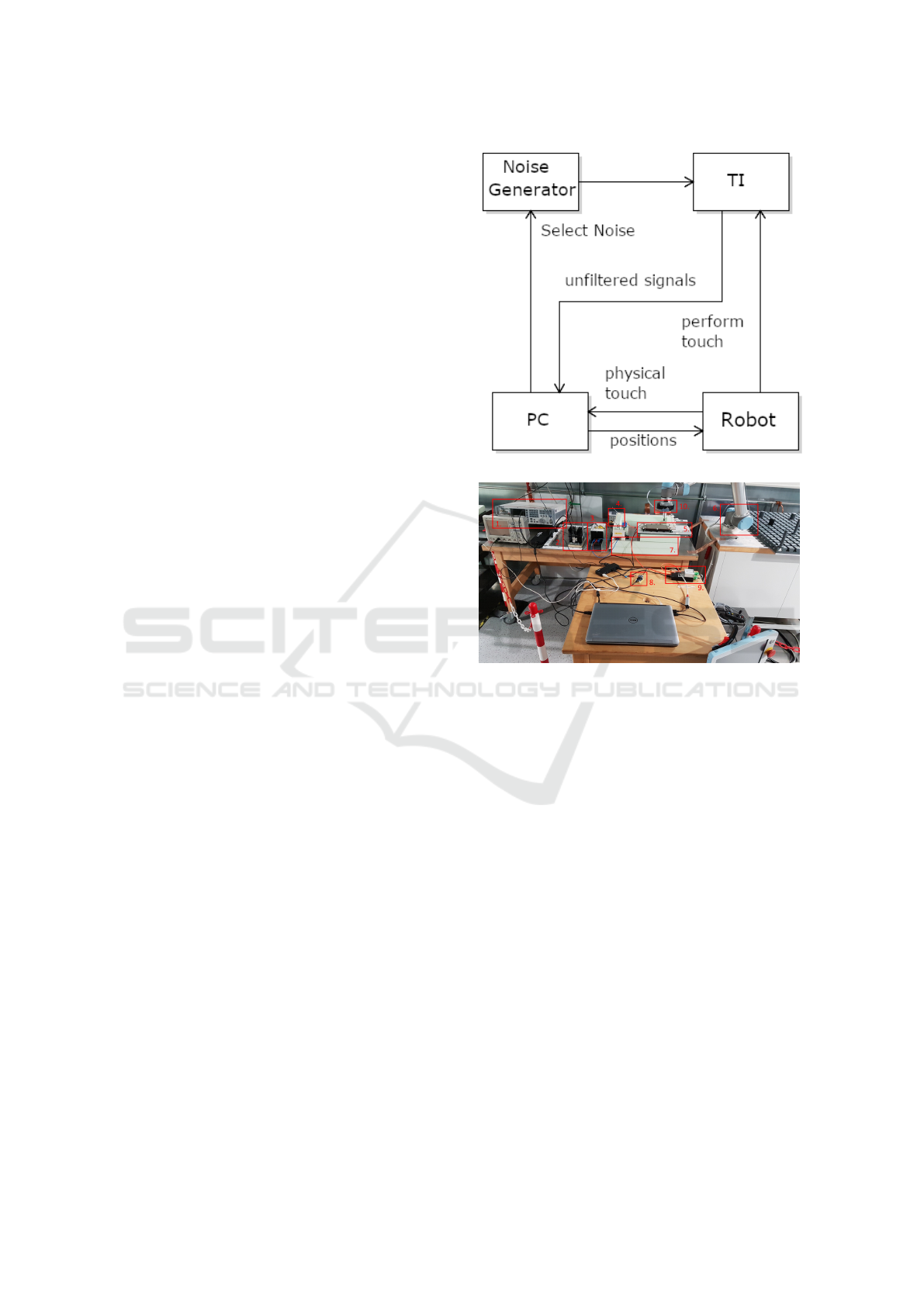
4 TEST BED
Within this section we describe the hardware set up
that we employed for our automatisation. On a high
level it consists out of a noise generator, a robot, the
TI, and a computer. The computer controls which
noise is introduced onto the TI and furthermore it de-
cides where the robot performs a physical touch. Our
robot is further equipped with a force sensor and thus
we are able to measure when exactly the robot has in-
teracted with the TI. Additionally the computer com-
municates with the TI. They can exchange both filter
parameters as well as sensed signals and touch events
detected by the TI.
(a) Abstract overview of our test bed.
(b) Concrete test bed in our lab.
Figure 2: Overview of the employed test bed.
A first feasible optimization approach using this
test bed would be to adjust the TI to certain filter pa-
rameterization, then to evaluate these parameters (in-
troduce noise, touch events and measure the TI’s out-
put). We decided against such an approach out of the
following reasons:
• Many search based optimization methods evalu-
ate different solutions iteratively (Neumann and
Witt, 2010) and thus prolonged evaluations on the
actual hardware would be necessary.
• Previously measured signals are thrown away af-
ter one parameter set has been examined.
Instead of such an online optimization approach we
measure touch events of differing duration once (in-
cluding different noise levels). This leads to the set
up described in Figure 2 (a).
In our later experiments we perform an offline op-
timization using the aforementioned data. Whenever
we intend to examine a parameter set we run a simula-
tion of the filterchain (instantiated with the parameter
set and applying it to the measured data). For our in-
An Evolutionary Calibration Approach for Touch Interface Filter Chains
31

dustrial partners we observed that the digital signal
processing part is usually written in C/C++ and can
be recompiled rather easily for an ordinary computer.
Thus the effort to acquire a simulation is manageable.
It is worth mentioning that for our industrial partners
corresponding hardware filters are usually employed
before the software filters are applied and thus this set
up is also feasible for these situations (the simulation
starts with the output of the signal filtered by the hard-
ware).
The concrete test bed located in our laboratory is
shown in Figure 2 (b). The noise generator consists
out of several components: a Teseq NSG 4070 sig-
nal generator (1.) that is coupled with 6 dB damper
(2.) which gives the damped noise signal onto a cou-
pling network (3.). The coupling network introduces
the noise signal onto the power supply (4.) which
feeds the TI (5.). Our six-axis robot is shown in (6.).
The IEC norm (IEC, 2009) further requires an iso-
lated test setup which we achieve using several layers
of polystrol (7.). The communication interface of (8.)
can be used to set filter parameters if need be and the
communication interface shown in (9.) is used to grab
the raw signals as described in 2 (a). The box number
10 contains the force sensor.
5 CALIBRATION APPROACH
Within this section we introduce the necessary nota-
tion to describe the calibration task. Furthermore the
underlying optimization approach is explained. Addi-
tionally we illustrate the GA that we use throughout
our experiments.
5.1 Optimization Problem
At each time stamp t the TI samples a signal value
s(t). The value is then processed by a configurable
filterchain and a decision is made if there has been
a touch event or not. Let p be the parameter vec-
tor which configures the filters. In our case we con-
sider filter elements whose parameters are integers
and thereby p ∈ Z
d
where d denotes the number pa-
rameters. Further let f (s(t), p) be the binary output of
the filterchain (touch yes or no).
In order to fit the filters we use a sample of fixed
length N. The goal of the calibration is that f (s(t), p)
should be equal to the actual touch events a(t) (mea-
sured by the robot’s force sensor).
A given calibration p should be capable to detect
the introduced touch events which can be measured as
follows:
T P(p) =
|{0 ≤ t ≤ N|a(t) = 1 ∧ a(t) = f (s(t), p)}|
|{0 ≤ t ≤ N|a(t) = 1}|
(1)
The measure T P is an adaption of the true positive
rate to the use case.
Additionally the configured filter should detect
correctly if there was no touch event at all:
T N(p) =
|{0 ≤ t ≤ N|a(t) = 0 ∧ a(t) = f (s(t), p)}|
|{0 ≤ t ≤ N|a(t) = 0}|
(2)
T N corresponds to the true negative rate.
Our objective function is based on the two afore-
mentioned measures and can be computed as follows:
T P(p) + T N(p)
2
(3)
The factor 2 is used for a normalization and thus its
values range from 0 (worst) to 1 (best). If a value of
1 is achieved then the calibrated filterchain does not
miss a single touch event and it correctly recognizes
if no touch is introduced onto the device. If a touch
event is not detected or a touch event is falsely rec-
ognized, the value declines. Thus the objective func-
tion is to be maximized. It is worth mentioning that
the objective function is also coined fitness function in
evolutionary computation (Neumann and Witt, 2010).
We follow this naming convention in the succeeding
sections.
5.2 Genetic Algorithm
Genetic algorithms are population based metaheuris-
tics (Holland, 1992). Each element of the population
represents a solution for the underlying optimization
problem. During an iteration of a GA, two individuals
are drawn from the population which is coined selec-
tion. These solutions are then combined to create two
new solutions. This step is called crossover. Further,
these two solutions may be changed randomly which
is named mutation. After these operations the new so-
lutions will be inserted into the population. The popu-
lation has a fixed boundary. A deletion mechanism is
triggered when the capacity is reached (to make space
for new solutions). This process is repeated until a
stopping criterion is reached. Within this work we
stop when a fixed search time is exhausted. A corre-
sponding pseudocode is displayed in Algorithm 1.
For our GA we use a k-tournament selection. Thus
we draw k random solutions from the population and
choose the one with the highest fitness. This is re-
peated twice in order to get two solutions x and y
that will be used for the crossover operation. For
the latter we use a one-point crossover to generate
ICINCO 2021 - 18th International Conference on Informatics in Control, Automation and Robotics
32

two new solutions. The operator chooses an integer
r from {1, 2, .., d} uniformly at random which serves
as a breakpoint. The first child
˜
x receives the first r
entries from x and the last d − r entries from y:
˜
x
i
=
(
x
i
i ≤ r
y
i
i > r
(4)
For the second child
˜
y this is reversed (first r en-
tries from y, remaining entries from x).
We apply a creep mutation. Each element gets a
new value with a probability of µ. Further, an eli-
tist deletion mechanism is used and thus the elements
with the worst fitness are deleted.
Algorithm 1: GA as pseudocode.
1 P = create initial population()
2 while stopping criterion is not met do
3 Choose x, y from P via selection
4 Create
˜
x,
˜
y from x, y via crossover
5 Mutate
˜
x,
˜
y using µ
6 insert
˜
x,
˜
y to P
7 if population capacity exceeds limit then
8 perform deletion
9 end
10 return one of the best solutions of P
We initialize our population entirely at random,
but we take the datatype of each filter parameter into
account. For example if a parameter is modelled as
an unsigned integer which is saved in a byte then we
draw a value from 0 to 255 uniformly at random.
6 EVALUATION
Within our experiments we rely on the generic fil-
terchain used in the TIs of BSH Hausger
¨
ate GmbH
which is Europe’s biggest producer of home appli-
ances. The company develops and sells devices un-
der the brands Bosch, Siemens, Neff, Gaggenau and
many more. The filterchain is used throughout their
products (e. g. dishwashers, ovens, coffee machines).
We rely both on simulated data as well as on data from
a TI which is a part of a cooktop. The signal process-
ing chain itself consists out of six with each other con-
nected building blocks (e. g. a low pass filters). Each
block has at least one parameter which may be config-
ured. In total our GA has to calibrate 15 parameters.
We repeat every experiment that we conduct thirty
times and represent averaged results. Furthermore we
give the GA a search time of two hours. For our ex-
periments we used a Dell OptiPlex XE3 with 32GB
RAM and an Intel i7 8700 processor and it was not
used for anything else during the evaluation.
Table 1: High level fitness overview. Values rounded to the
fifth digit.
train dataset test dataset
Maximum 0.94895 0.94961
Minimum 0.68822 0.59832
Mean 0.86883 0.82119
Standard deviation 0.07271 0.06730
1. Quartile 0.81703 0.77135
Median 0.89924 0.83441
3. Quartile 0.92848 0.87174
6.1 Hyperparameter Study
The chosen hyperparameters can affect the perfor-
mance of metaheuristics such as a GA (B
¨
ack et al.,
1997). Thus we decided to evaluate the effect of dif-
ferent hyperparameter combinations on the GA’s per-
formance. For k we consider {5, 10, ..., 35}, for the
population sizes |P| {250, 500, ..., 1500} and for the
mutation probability µ {0.01, 0.02, ..., 0.06}.
We use an ideal, simulated signal s(t) that contains
no noise at all. We do this by creating touch events of
different lengths. We also create phases of different
length where no touch has been introduced. The sig-
nal is a sequence of 100 touch ON and touch OFF
phases. It starts and ends with an OFF phase. The
ON phase has a random duration of between 30 and
80 time stamps. We use the 10 starting and 10 ending
time steps to let the signal level rise from OFF to ON
and from ON to OFF respectively. This modelled as
linear function, for example for the rising signal:
s(t) = OFF +
ON
10
∗ (t −t
0
) (5)
where t
0
is the start of increasing signal slope. The
length of the OFF phase is also created randomly and
ranges from 50 to 500 time steps. Thus longer sec-
tions where no one interacts with the TI can be simu-
lated. For our test dataset we perform the same gen-
eration procedure but only create 10 touch ON and
Touch OFF phases.
In our later experiments we rely on different data.
Thus the hyperparameters that we choose within this
study are not overfitted to one of the later datasets.
We give a short summary about the fitness values
achieved in Table 1. We computed the table based on
the average values achieved for each hyperparameter
combination. It displays minima, maxima, quartiles,
mean values and the standard deviation on the train-
ing and test dataset. We can observe a large range
of more than 25 percent for the achieved fitness val-
ues on both datasets. This underlines the sensitivity
of our GA with respect to its hyperparameters. The
An Evolutionary Calibration Approach for Touch Interface Filter Chains
33

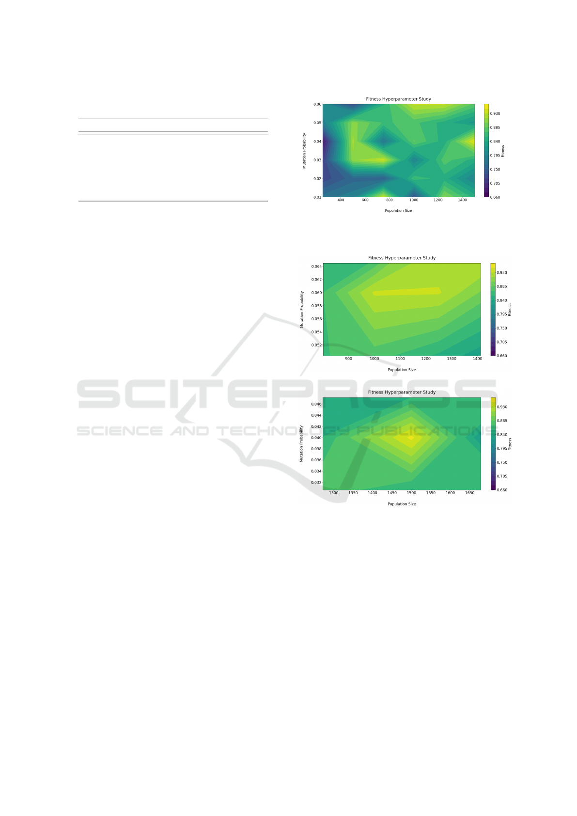
Table 2: Top five hyperparmeter combinations and their me-
dian fitness.
k µ |P| fitness train fitness test
35 0.05 750 0.94895 0.93637
30 0.03 750 0.94875 0.93647
30 0.03 250 0.94874 0.93655
30 0.06 1000 0.94839 0.94961
25 0.05 1250 0.94040 0.94788
majority of the fitness range is covered by half of the
considered combinations as we can see by the quar-
tiles displayed. The fitness values of the remaining
combinations are closer. This variability can also be
seen in the standard deviation which is between 6.7
and 6.9 percent. On the test dataset the mean and the
median are similar but on the training dataset there is
a gap of 5 percent between the two due to outliers.
The prior analysis lacks the link to the combina-
tions’ location in the hyperparameter space. We fo-
cus first on the top five training fitness combinations
due to the high dimensionality (mutation probability,
population size, tournament k, fitness value). We dis-
played these in Table 2. On these we can see that
a high fitness value on the training data set can lead
to high values on the test dataset. For example the
parameter combination with the highest test fitness
is also within the table. The worst of our top five
combinations is still better than the aforementioned
3.Quartiles which further underlines the GA’s sensi-
tivity to the chosen hyperparameters. Generally our
GA benefits from a high k and thus a longer search
through the population to find a parent is performed.
For the mutation probability we can observe medium
and high values. For the population size we can notice
nearly the full considered range of values. It is worth
mentioning that on the top five worst hyperparameter
combinations the population sizes and mutation prob-
abilities are low and the tournament k is high. The
weak performance can be due to a lack of diversity in
the population.
Based on Table 2 we fixed k to 30 and plotted the
fitness landscape (on the test dataset) in Figure 3 (as
the best test set performance is achieved with k = 30
and a good performance on the training dataset can
also be observed). There is a small sweetspot for pop-
ulation sizes of 500 to 750. Furthermore we can iden-
tify higher fitness plateaus on the right and on the top
of the plot. We decided to analyse these regions fur-
ther. The corresponding plots are shown in Figures
4 (a) and (b). We can see that both regions are an
isolated local optima and no gain in fitness can be ob-
served if we go further in either direction.
Figure 3: Fitness values on the test dataset for tournament
k = 30.
(a) Fitness region on the top.
(b) Fitness region on the right.
Figure 4: Fitness at the corner regions.
Based on our hyperparameter study we set k to
30, the mutation probability to 0.06 and the maxi-
mum population size to 1000 for the succeeding ex-
periments. We decided to use this combination as it
achieved the highest fitness value on the test dataset
and is close to the best performance on the training
dataset (there is only a difference of 0.00056).
6.2 Simulated Noise
We extend our setting from the hyperparameter study
by introducing noise to the simulated signal. We de-
cided to use white noise which is common in signal
ICINCO 2021 - 18th International Conference on Informatics in Control, Automation and Robotics
34

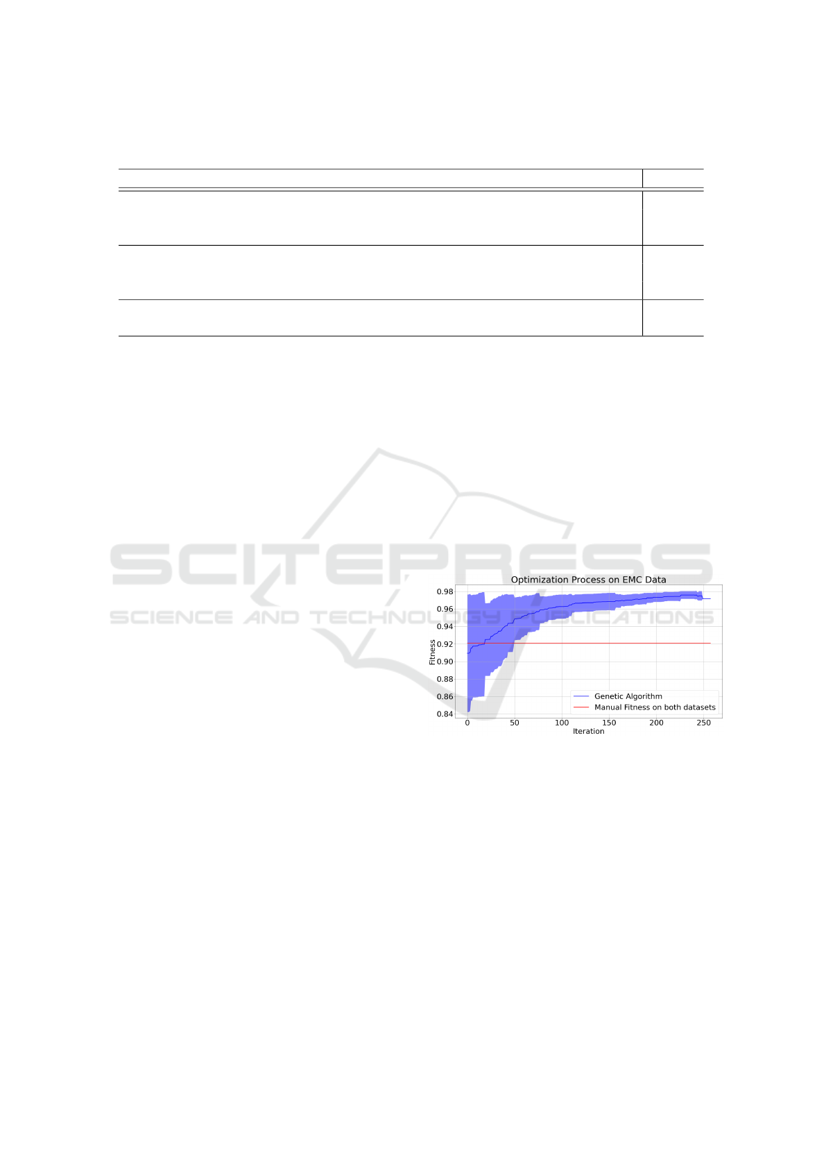
Table 3: Results for different Gaussian noise and EMC noise. Iteration related metrics are rounded to integers. The remaining
measures are rounded to the fifth digit.
σ = 10 σ = 15 σ = 20 σ = 25 EMC
fitness of manual calibration (test dataset) 0.96512 0.97109 0.96450 0.96792 0.97081
median fitness GA (test dataset) 0.97763 0.98954 0.99141 0.99249 0.97560
deviation fitness GA (test dataset) 0.15849 0.14793 0.00635 0.08988 0.00851
fitness of manual calibration (train dataset) 0.96495 0.96383 0.96356 0.96013 0.76109
median fitness GA (train dataset) 0.97987 0.98987 0.99127 0.99164 0.97174
deviation fitness GA (train dataset) 0.00401 0.00400 0.00107 0.00131 0.00579
median of iterations until human level 129 142 75 67 67
standard deviation of iterations until human level 81 154 68 65 68
processing (Tuzlukov, 2018) and time series analysis
(Cressie and Wikle, 2015).
We employ the noise in our simulation by gener-
ating Gaussian distributed random variables ε(t) with
mean zero and standard deviation σ and adding them
to s(t). Thus we observe the following noisy signal:
s(t) + ε(t) (6)
We employ different sigmas {10, 15, 20, 25}. Hence
we consider four different training datasets here. It
is worth mentioning that the noise-free signal s(t)
ranges from 0 to 100 in our simulation. Each train-
ing and test dataset contains the same number of ON
and OFF phases as in the hyperparameter study. Fur-
thermore the durations of each phase are created in
the same way.
We display the achieved results in columns 2 to
5 of Table 3. We display the different median fitness
values achieved (on both train and test dataset). Addi-
tionally the table holds the fitness values achieved by
the manual calibration. We can see that if we consider
the median value the GA approach always leads to
better results on both the training and the test dataset.
However, one should keep in mind that the GA does
not always have a constant output as can be derived
from the non-zero standard deviation. Thus we ad-
ditionally perform a Wilcoxon ranksum test in order
to verify our hypothesis. It is worth mentioning that
this statistical test has no preconditions that need to be
checked. We measured a p-value below 10
−30
which
we regard as significant and thus we infer that in this
experiment the GA’s parameters lead to higher fitness
values than the manually determined ones.
Table 3 additionally contains information about
the number of iterations necessary until the evolution-
ary algorithm surpasses the human approach’s perfor-
mance on the datasets. Generally we can observe that
the GA needs a rather low number of iterations until
it exceeds. The magnitude depends on the considered
noise level which we confirmed using an additional
Friedman test (with a significance level of 0.05).
6.3 Electromagnetic Noise
Within our last experiment we switch our focus on
real data collected from our lab. We introduced sev-
eral touch events using our robot and focused on a
noise family which is known as injected current in
electrical engineering. For details on this test we re-
fer the reader to the corresponding IEC standard (IEC,
2009).
Our EMC dataset consists out of 129,759 samples
and we used the first 90 percent for training and the
remaining 10 percent for validation. It contains 202
ON and OFF phases.
Figure 5: Learning Process of the GA plus minus standard
deviation on the EMC data. The plot further contains the
fitness of the manual calibration on both the training and
validation dataset.
We display the results in the column “EMC” of
Table 3. Again we can observe that our GA leads
to more precise parameters on both the training and
the test dataset. We once more perform an additional
Wilcoxon ranksum test to verify this hypothesis. We
examine the nullhypothesis “The manual calibration
is superior to the calibrations found by the GA on the
training and the test dataset”. We computed a p-value
of less than 10
−8
which we regard as significant. Thus
we reject the nullhypothesis and accept the alternative
hypothesis that the GA leads to more precise calibra-
tions. It is worth mentioning that this low p-value is
An Evolutionary Calibration Approach for Touch Interface Filter Chains
35

not only due to the performance gap on the training
dataset. If we would examine both datasets in isola-
tion then we could still observe a p-value of less than
10
−6
on the training dataset and of about 0.01 on the
test dataset.
We already mentioned a considerable perfor-
mance gap between the manual calibration and the
ones found by our GA if the training dataset is con-
sidered. There is a sequence of touch events in the
dataset with high noise levels that the TI using the
manually determined parameters fails to recognize.
However, this is not the case if we employ the param-
eters found by our GA (the TI is capable of detecting
these events using the GA’s calibration).
For our EMC experiment we once more can see
that the GA outperforms the human at this task rather
quickly. The median iterations necessary to achieve
this is less than one hundred. However, we decided
to give a more fine-grained overview on the learning
process in Figure 5. It displays the average fitness
plus minus its standard deviation at each step. We ad-
ditonally added the performance of the manually de-
termined calibration (on the training- and testdataset)
to the plot.
We can observe a large variation at the beginning
which is gradually declining over time. This is due
to the creation of several hundred random solutions
for initialization of the population. This might lead
to starting solutions that already have decent fitness
values. Generally the GA already starts at rather high
fitness values (of about 90 percent) which it can grad-
ually improve. Furthermore we can see that there is
some variation in the number of iterations performed
in the two hours (as there is a fitness drop after about
240 iterations which does not happen if one run of
our elitist GA is evaluated in isolation). Even though
GA has search time of two hours it only performs up
to 250 iterations per search. This is due to the com-
putational cost of the fitness function. Whenever we
want to evaluate a solution we have to process about
117,000 samples of the training data set. For each
sample the signal processing component must be exe-
cuted. Thus an evaluation of the fitness function costs
several seconds execution time.
6.4 Qualitative Remarks
In our experiments we could show that our method is
capable of outperforming a manual approach and we
could achieve recognition rates of 97 to 99 percent
on the respective validation set. However, we did not
discuss if these seemingly high values can be consid-
ered as good or not. Thus we take a closer look at the
performance achieved within this subsection.
Figure 6: Example of prolonged touch events due to a low
pass filter (on the EMC data).
For most samples we observed the behaviour
shown in Figure 6. The plot displays the output of
the calibrated filter chain as well as the touch events
detected using the force sensor. In this example we
can see that our calibration detects touch events cor-
rectly but prolongs them. The examined filterchain
contains a low pass filter to tackle noise (Rao and
Swamy, 2018). This filter element has the side ef-
fect that it delays the signal slightly which explains
this observation. Our fitness level works at the sample
level which explains why we do not achieve a recog-
nition rate of 100 percent. We sample fast (at about 10
ms) and thus we deem these prolonged touch events
as acceptable. In fact the highest prolongation that we
found was about 150 ms.
It is worth mentioning that the parameterization
provided by the GA cannot deal with unlimited noise.
If the noise level becomes too high then we observed
that our calibration may miss out touch events. How-
ever, we made similar observations with the manual
calibration that fulfills the IEC standard. Thus we fo-
cused on a setting that satisfies the industry standard
within the experiments.
7 FUTURE WORK
Within this study we focused on touch events. How-
ever, modern TIs also offer more complicated features
such as multitouch recognition capabilites (e. g. for
zooming in and out using two fingers). We will ex-
amine if our GA is also capable to provide robust pa-
rameterizations for such methods.
A current trend in manufacturing is to move from
a fixed set of parameters to adaptive ones (Heider
et al., 2020). The most promising parameters are cho-
sen according to the system’s state and this enables
the configuration to be more specialised. In our case
we would extend the TI software by a noise detection
and classification system which can be used as a de-
ICINCO 2021 - 18th International Conference on Informatics in Control, Automation and Robotics
36

cision basis for a set of trained parameters.
From an engineering point of view we want to fur-
ther improve the solution’s degree of automatization
by employing continuous integration (CI) techniques
(Smart, 2011). CI focuses merging code of individ-
ual programmers frequently. We intend to use the
methodology to automatically test and perhaps recali-
brate the TI whenever new source code is introduced.
8 CONCLUSION
Modern touch screens are both electrical sensors and
digital signal processing units. Often the signal
processing part consists out of multiple components
which must be calibrated precisely in order to as-
sure proper functionality. Additional legal obligations
such as electromagnetic compatibility must be met by
a calibration. We provided automated solution to de-
termine robust parameterizations for the signal pro-
cessing approach. We could not only erase the pain
of calibrating the device by hand, we could also show
that our method leads to a superior calibration.
ACKNOWLEDGEMENT
We would like to thank Mircea Barbu and Carsten
Fischer for supporting and sponsoring this research
project. Furthermore we would like to express our
gratitude towards our BSH colleagues that helped us
understanding the use case and setting up the test bed.
REFERENCES
Arakawa, M., Yamashita, Y., and Funatsu, K. (2011). Ge-
netic Algorithm-based Wavelength Selection Method
for Spectral Calibration. Journal of Chemometrics,
25(1):10–19.
Atmel (2020). Atmel Max Touch Overview.
http://ww1.microchip.com/downloads/en/DeviceDoc/
45071A maXTouch Portfolio E US 060514 Web.
pdf. [Online; accessed 3-December-2020].
B
¨
ack, T., Fogel, D. B., and Michalewicz, Z. (1997). Hand-
book of Evolutionary Computation. IOP Publishing
Ltd., GBR, 1st edition.
Cressie, N. and Wikle, C. (2015). Statistics for Spatio-
Temporal Data. Wiley.
Doerr, A., Nguyen-Tuong, D., Marco, A., Schaal, S., and
Trimpe, S. (2017). Model-based policy search for au-
tomatic tuning of multivariate pid controllers. In 2017
IEEE International Conference on Robotics and Au-
tomation (ICRA), pages 5295–5301.
EU (2014). Directive 2014/30/EU. https:
//ec.europa.eu/growth/single-market/european-
standards/harmonised-standards/electromagnetic-
compatibility en. [Online; accessed 7-December-
2020].
Haga, H. and Suehiro, A. (2012). Automatic test case gen-
eration based on genetic algorithm and mutation anal-
ysis. In 2012 IEEE International Conference on Con-
trol System, Computing and Engineering, pages 119–
123.
Harding, S., Leitner, J., and Schmidhuber, J. (2013). Carte-
sian Genetic Programming for Image Processing,
pages 31–44. Springer New York, New York, NY.
Heider, M., P
¨
atzel, D., and H
¨
ahner, J. (2020). Towards
a Pittsburgh-Style LCS for Learning Manufacturing
Machinery Parametrizations. In Proceedings of the
2020 Genetic and Evolutionary Computation Confer-
ence Companion, GECCO ’20, page 127–128, New
York, NY, USA. Association for Computing Machin-
ery.
Holland, J. H. (1992). Genetic Algorithms. Scientific Amer-
ican, 267(1):66–73.
IEC (2009). 61000-4-6: Testing and Measurement
Techniques – Immunity to conducted Distur-
bances, induced by radio-frequency Fields.
https://www.iecee.org/dyn/www/f?p=106:49:0::::
FSP STD ID:18793. [Online; accessed 3-December-
2020].
Man, K. F. and Tang, K. S. (1997). Genetic Algorithms for
Control and Signal Processing. In Proceedings of the
IECON’97 23rd International Conference on Indus-
trial Electronics, Control, and Instrumentation (Cat.
No.97CH36066), volume 4, pages 1541–1555 vol.4.
Margraf, A., Stein, A., Engstler, L., Geinitz, S., and Hah-
ner, J. (2017). An Evolutionary Learning Approach
to Self-configuring Image Pipelines in the Context of
Carbon Fiber Fault Detection. In 2017 16th IEEE In-
ternational Conference on Machine Learning and Ap-
plications (ICMLA), pages 147–154.
MATT (2020). MATT ROBOT - The ultimate Touchscreen
Testing Tool. https://www.mattrobot.ai/. [Online; ac-
cessed 4-December-2020].
Millo, F., Arya, P., and Mallamo, F. (2018). Optimization of
Automotive Diesel Engine Calibration using Genetic
Algorithm Techniques. Energy, 158:807 – 819.
Neumann, F. and Witt, C. (2010). Bioinspired Computa-
tion in Combinatorial Optimization: Algorithms and
their Computational Complexity. Natural Comput-
ing Series, ISBN 978-3-642-16543-6. Springer-Verlag
Berlin Heidelberg, 2010.
OptoFidelity (2020). Touch Testing. https://www.
optofidelity.com/touch-testing/. [Online; accessed 4-
December-2020].
Rao, K. D. and Swamy, M. N. S. (2018). Digital Signal
Processing: Theory and Practice. Springer Publish-
ing Company, Incorporated, 1st edition.
Ryan, C., Tetteh, M. K., and Mota Dias, D. (2020). Be-
havioural Modelling of Digital Circuits in System Ver-
ilog using Grammatical Evolution. In Proceedings of
An Evolutionary Calibration Approach for Touch Interface Filter Chains
37

International Joint Conference on Computational In-
telligence.
Shafii, M. and De Smedt, F. (2009). Multi-Objective Cali-
bration of a distributed hydrological Model (WetSpa)
using a Genetic Algorithm. Hydrology and Earth Sys-
tem Sciences, 13(11):2137–2149.
Smart, J. F. (2011). Jenkins: The Definitive Guide. O’Reilly,
Beijing.
ST (2018). Getting Started with Touch Sensing Control
on STM32 Microcontrollers. https://www.st.com/
resource/en/application note/dm00445657-getting-
started-with-touch-sensing-control-on-stm32-
microcontrollers-stmicroelectronics.pdf. [Online;
accessed 10-December-2020].
Stegherr, H., Heider, M., and H
¨
ahner, J. (2020). Classifying
Metaheuristics: Towards a unified multi-level classifi-
cation system. Natural Computing.
TacticleAutomationInc (2020). Robotic Touch Panel
Tester – TakTouch 1000. https://tactileautomation.
com/shop/touch-panel-test-systems/robotic-touch-
panel-tester-taktouch-1000/. [Online; accessed
4-December-2020].
Tuzlukov, V. (2018). Signal Processing Noise. Electri-
cal Engineering & Applied Signal Processing Series.
CRC Press.
Walker, G. (2012). A Review of Technologies for Sensing
Contact Location on the Surface of a Display. Jour-
nal of the Society for Information Display, 20(8):413–
440.
Wu Zhizhou, Sun Jian, and Yang Xiaoguang (2005). Cal-
ibration of VISSIM for Shanghai Expressway using
Genetic Algorithm. In Proceedings of the Winter Sim-
ulation Conference, 2005.
ICINCO 2021 - 18th International Conference on Informatics in Control, Automation and Robotics
38