A Genetic Algorithm for HMI Test Infrastructure Fine Tuning

Lukas Rosenbauer

, Anthony Stein

and J

org H

ahner

BSH Hausger

ate GmbH, Im Gewerbepark B35, Regensburg, Germany

Artiﬁcial Intelligence in Agricultural Engineering, University of Hohenheim, Garbenstr. 9, Stuttgart, Germany

Organic Computing Group, University of Augsburg, Am Technologiezentrum 8, Augsburg, Germany

Keywords:

Automatization, Testing, Genetic Algorithm, Computer Vision.

Abstract:

Human machine interfaces (HMI) have become a part of our daily lives. They are an essential part of a variety

of products ranging from computers over smart phones to home appliances. Customer’s requirements for

HMIs are rising and so does the complexity of the devices. Several years ago, many products had a rather

simple HMI such as mere buttons. Nowadays lots of devices have screens that display complex text messages

and a variety of objects such as icons. This leads to new challenges in testing, the goal of which it is to ensure

quality and to ﬁnd errors. We combine a genetic algorithm with computer vision techniques in order to solve

two testing use cases located in the automated veriﬁcation of displays. Our method has a low runtime and can

be used on low budget equipment such as Raspberry Pi which reduces the operational cost in practice.

1 INTRODUCTION

HMIs enable customers to interact with a product.

They can be rather simple components such as rotary

knobs or sliders. Expensive devices can offer more

complicated HMIs such as voice control, gesture con-

trol, or touch displays which offer even more ways to

interact with a device.

These advances have led to new challenges in the

development of the aforementioned solutions. An es-

sential part of development is the veriﬁcation of the

product. The testing of HMIs has undergone se-

rious investigation from various perspectives. Ma-

teo Navarro et al. (2010) examine HMI testing from a

software engineering point of view and propose an ar-

chitecture for graphical user interface (GUI) testing.

Duan et al. (2010) developed a model-based approach

to achieve a high code coverage and to keep the de-

velopment cost in bounds. Howe et al. (1997) exploit

planning techniques in order to generate test cases for

GUIs using evolutionary methods. A genetic algo-

rithm was used by Rauf et al. (2011) to improve the

path coverage of GUIs.

The aforementioned approaches deal with the

question: How should HMI testing be done? With the

move from manual testing to automated testing, an-

other task is to provide the right tools for testers to im-

plement tests. Inadequate test infrastructure is respon-

sible for major economical losses (Hierons, 2005).

Thus it is a proﬁtable goal to provide testers with the

right testing equipment.

Within this work, we combine an evolutionary al-

gorithm with more traditional computer vision algo-

rithms to solve two use cases for the visual validation

of GUIs. Both deal with the identiﬁcation of GUI ele-

ments. The ﬁrst deals with the veriﬁcation of screens

from simulations or the framebuffer based on the de-

signer’s speciﬁcation. The latter does not require the

entire HMI as only the buffer and the CPU are neces-

sary. The second one is a part of the electronic com-

ponent test which has the goal to verify the software’s

behaviour combined with the hardware of the HMI.

There we try to recognize various icons.

Both problems could be solved by using artiﬁcial

neural networks. However, these have the downside

that the number of possible classes must be known

during the design time of the network (G

eron, 2017).

Usually testing is started early (Olan, 2003) and re-

quirements change during the lifetime of a project

(Nurmuliani et al., 2004) which might lead to frequent

redesigns and retrainings of the speciﬁed neural net-

work. Another downside is that usually an Nvidia

GPU must be acquired in order to have reasonable

runtimes (G

eron, 2017).

We deemed this as unfavorable and thus took a

look at more traditional computer vision methods

such as template matching or feature detectors that

do not have these downsides (Szeliski, 2010). On the

Rosenbauer, L., Stein, A. and Hähner, J.

A Genetic Algorithm for HMI Test Infrastructure Fine Tuning.

DOI: 10.5220/0010512803670374

In Proceedings of the 18th International Conference on Informatics in Control, Automation and Robotics (ICINCO 2021), pages 367-374

ISBN: 978-989-758-522-7

367

other hand, they require the correct calibration of for

example edge detection thresholds. In order to avoid

calibrating these parameters manually, we apply a ge-

netic algorithm (GA) to do this automatically.

Further, we provide a proof of concept that a GA

can be used to automatically ﬁne-tune computer vi-

sion methods for HMI testing. In our experiments

we show that our calibrated recognition methods are

not only able to correctly identify GUI elements, but

that our calibration approach also needs a compara-

bly small amount of data. Furthermore, our experi-

ments reveal that the designed methods have a rather

low runtime which enables us to test more screens and

the designed approach can also be used on low-budget

boards such as Raspberry Pi.

In Section 2 we discuss related work. We provide

a more detailed description of the use cases in Sec-

tion 3. Afterwards, several computer vision methods

are introduced that we are going to calibrate (Section

4). This is followed by a description of our ﬁtness

function and GA (Section 5). In Section 6 we per-

form a series of experiments that verify our approach.

We close the paper with a conclusion (Section 7).

2 RELATED WORK

HMI testing got into the focus of several compa-

nies. For example Froglogic’s Squish framework or

Bosch’s Graphics Test System offer various function-

alities for GUI veriﬁcation. Some of these software

products enable test engineers to use trained machine

learning models such as neural networks for optical

character recognition (Froglogic, 2020). Others re-

quire the manual calibration of algorithmic parts for

the recognition of GUI elements, for example the test

system of the company Zeenyx (2020). Some of these

visual testing frameworks have found their way into

various companies (Al

egroth et al., 2016).

From a scientiﬁc point of view, the visual veriﬁ-

cation of GUI elements such as icons is an applica-

tion of computer vision (CV). This problem is known

as object recognition (Szeliski, 2010). This can be

achieved by using artiﬁcial neural networks (G

eron,

2017). There are also possible solutions outside of

machine learning such as feature detectors (Lowe,

1999). It is worth mentioning that these CV method-

ologies also require a precise calibration of the un-

derlying parameters in order to work properly. Fur-

ther, the quality of the image recognition algorithms

has been detected as key issue in visual testing and

several enterprises encountered issues with the frame-

works available (Al

egroth et al., 2013).

GAs have been used for a variety of calibration

tasks such as spectroscopy (Attia et al., 2017) and en-

ergy models (Lara et al., 2017). We think that these

positive results indicate that a GA might also be use-

ful to ﬁne-tune CV methods for HMI veriﬁcation. It

is also worth mentioning that there a variety of alter-

native evolutionary techniques as documented in the

survey of Stegherr et al. (2020). However, due to the

aforementioned successful usages of GAs we decided

to start with this class of metaheuristics.

3 PROBLEM DESCRIPTION

Within this section, we introduce our two use cases.

We provide several example images to ease under-

standing and show how they can be solved using pure

CV.

3.1 Veriﬁcation on a Pixellevel

Before the images of an application are displayed,

they are usually held in a framebuffer. When it is

time to be shown on the display then the currently

displayed image will be deleted. Afterwards, the next

screen is loaded from the buffer to the display. During

this process errors might occur as pixels are not prop-

erly loaded, old pixels are not deleted, or the image al-

ready contains errors in the buffer. We displayed such

a case that we encountered in a company in Figure 1

where the word “Wecker” contains a pixel error (some

pixels of characters are black but should be white).

In order to detect pixel errors, template match-

ing (TM) can be applied Szeliski (2010). TM uses

an example image called template and compares it to

the image of an application. If both images are close

enough in terms of a similarity measure or distance,

then it is regarded as a match. TM can also be used

to validate parts of the application’s output. In our

example we discovered the error by rendering an im-

age containing the word “Wecker” and sampling the

screen.

There are several ways to acquire an exemplary

image that can be used as a template. One possibil-

ity is to use the designer’s speciﬁcation of individual

screens, another one is to use a test oracle (Ammann

and Offutt, 2016) which proposes the correct screen

based on the current GUI state. Due to technical lim-

itations there might still be some differences between

the template and the application. These minor differ-

ences can be tolerated and the screen can be seen as

valid. For example, the designers might deﬁne the

user interface’s colors in a format that uses one byte

per color channel (888 format) and the HMI uses a

686 format (6 bits for red, 8 bits for green, 6 bits for

ICINCO 2021 - 18th International Conference on Informatics in Control, Automation and Robotics

368

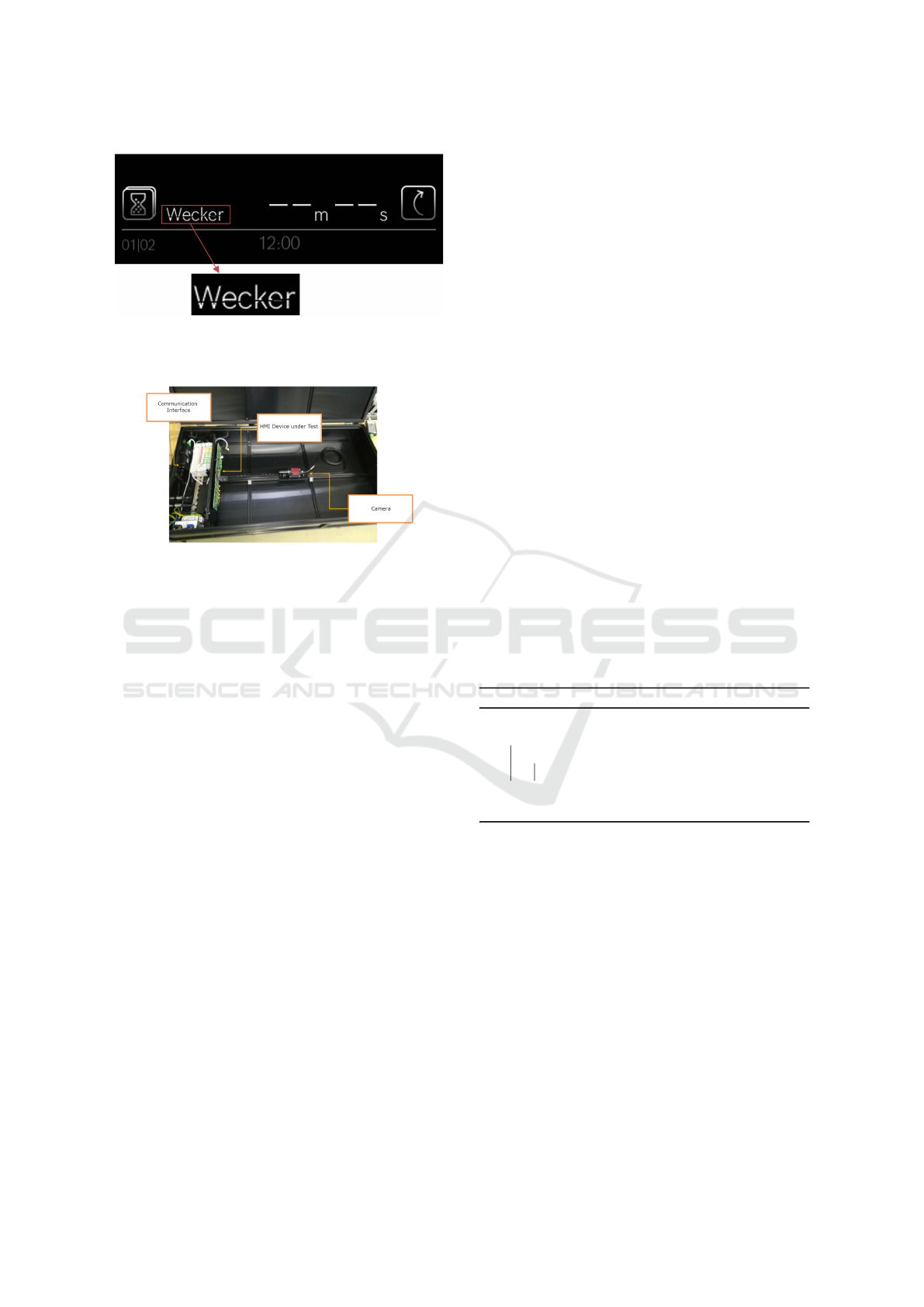
Figure 1: Example of a pixel error of an user interface. The

word “Wecker” contains pixel errors as some of the white

pixels are missing.

Figure 2: Example of a possible test environment for the

component test of an HMI.

blue) to save memory. Such memory saving color

formats are widespread in embedded systems (Mar-

wedel, 2010) and a transformation from the 888 for-

mat to the 686 format is lossy.

TM requires test engineers to set tolerances or

scale levels for the template. A too high tolerance

leads to failures that go undetected in automated tests.

An overly low tolerance can lead to false negative

tests. The tolerances may differ from region to region.

Thus the goal of this use case is to automatically set

the correct thresholds for TM.

3.2 Component Test

Component testing is a branch of veriﬁcation that lim-

its its scope to a certain part of the system. An HMI

can consist out of hardware and software. Both must

interact properly in order to satisfy customers. For

example, if a user selects a program on a dishwasher,

corresponding options should be displayed.

A possible approach for a corresponding test envi-

ronment is displayed in Figure 2. It consists out of a

camera to make images of the display, the HMI which

is to be tested, and a communication interface which

can be used to manipulate its state. We packed these

components in a black box in order to avoid side ef-

fects due to illumination. It is worth mentioning that

we are not the ﬁrst to evaluate a hardware using a

camera. For example, Ramler and Ziebermayr (2017)

used a camera-based testbed to verify the behaviour

of a mechatronic system.

Images taken via camera contain a certain amount

of noise due to the environment or the camera itself.

Further, the HMI may not be parallel to the lens. This

leads to slightly rotated GUI elements. A CV ap-

proach to tackle these problems are feature detectors

such as SIFT (Lowe, 1999) which can be used to rec-

ognize rotated objects. Furthermore, a raw TM is also

not sufﬁcient since GUI elements will most likely not

have the same scale as the template. In this use case

we will ﬁne-tune a CV method which combines fea-

ture detectors and TM.

4 COMPUTER VISION

ALGORITHMS

Here we introduce two basic CV algorithms that are

suitable for our two use cases, but they require the

ﬁne-tuning of certain parameters which we will do

later on using a GA.

The ﬁrst one is a simple template matcher de-

scribed in Algorithm 1. It samples the given image

using a sliding window with a step size of one pixel. If

the patch is similar enough then it returns true. There

can be several thresholds depending on the region of

interest (ROI) of the screen. In our later experiments

we will use the cosine similarity (Singhal, 2001).

Algorithm 1: Template matcher based on Szeliski (2010).

input : Image i, Template T

1 while Sample S left do

2 if similarity(S, T) > Threshold then

3 return True;

4 end

5 return False;

We further examine a feature-based approach

which is based on oriented fast and rotated brief

(ORB) (Rublee et al., 2011) and TM. We chose

ORB over SIFT and SURF as it is a non-patented

method which enables commercial use without li-

censing costs. Further, ORB is available in the well-

known open source library OpenCV (OpenCV.org,

2020).

We once more sample the given image. ORB com-

putes image features that are represented as bit vec-

tors which can be compared to each other using the

Hamming similarity (Rublee et al., 2011). For every

patch we calculate the k best matches between the fea-

ture of the object to search for and the image to ex-

amine. Further, the average µ of these similarities is

computed. Additionally we scale the template to var-

A Genetic Algorithm for HMI Test Infrastructure Fine Tuning

369

ious sizes, compare it with the patch, and return the

highest cosine similarity γ. If the following condition

holds we interpret that as a “found”:

β · µ + (1 − β) · γ > threshold (1)

where β is a real number between zero and one. It

controls the inﬂuence of TM and ORB on the classi-

ﬁcation result.

We summarized this process for one sampled

patch in Algorithm 2. Later on our GA will learn the

number of scale levels, the scale increment, β, k, and

the threshold. These can once more vary from ROI to

ROI.

Algorithm 2: Object recognition with TM and ORB.

input : Patch p, Template T

1 t feat = ORB features(T)

2 p feat = ORB feature(p)

3 k best = get k best matches(p feat, t feat)

4 µ = mean(k best similarities)

5 tm similarities = { }

6 for i in {-scale levels,...,scale levels} do

7 // scale to 1 + i * scale inc times its size

8 scaled temp = scale(T, 1 + i * scale inc)

9 // compute cosine similarity

10 sim = cos sim(p, scaled temp)

11 append sim to tm

similarities

12 end

13 γ = max(tm similarities)

14 if β · µ + (1 − β) · γ > Threshold then

15 return True;

16 return False;

5 EVOLUTIONARY FINE

TUNING

Evolutionary heuristics such as genetic algorithms

can be used to solve a variety of optimization ap-

proaches and were originally introduced by Holland

(1992). Here we use a GA for ﬁne-tuning existing

CV methods. Thus we differ from GP approaches as

these intend to optimize the structure of a CV process.

Within this section, we introduce a ﬁtness function

and a GA for our use cases.

5.1 Fitness Function

The design of our ﬁtness function has been inspired

by the benchmarking of information retrieval systems

such as search engines. The capability of a search en-

gine to answer a query can be evaluated using a set of

documents. Only a part of the documents are relevant

for the query. The search engine returns a subset of

the documents that it regards as important. The search

engine’s answer is then benchmarked by the number

of relevant and irrelevant documents that it returned

(Baeza-Yates and Ribeiro-Neto, 1999).

If an object recognition algorithm examines a set

of images then it should only detect GUI elements that

are available or in other words: There should be no

false positives. This can be examined using the preci-

sion P(·, ·) of an object recognition algorithm A for a

set of images S:

P(A, S) = 1 −

|out(A, S)\ ob(S)|

|out(A, S)|

(2)

where ob(S) represents a list containing the objects on

the set of images and out(A, S) represents a list con-

taining the objects that the algorithm claims to be on

the images. The elements of both lists are tuples of

the form (i, ob) where i is an image of S and ob is an

object. P ranges from zero to one. The best possi-

ble value of one indicates that an algorithm only de-

tected objects that were actually on the given images.

A value lower than one indicates that the algorithm

detected objects that are not there. In our analogy the

precision measures the amount of relevant documents

among the retrieved ones.

Further, a recognition method should not miss any

object. This can be measured via the recall R(·, ·):

R(A, S) =

|ob(S) ∩ out(A, S)|

|ob(S)|

(3)

Its values also range from zero to one. A value of

one means that the method found all available objects.

A smaller value indicates that the algorithm missed

something. In information retrieval it is used to quan-

tify the amount of relevant documents found by the

method.

We combine both quality measures into one ﬁtness

function F(·, ·):

F(A, S) =

P(A, S)+ R(A, S)

(4)

We divide both values by two in order to norm the

ﬁtness values. Thus it also ranges from zero to one.

A perfect algorithm that never misses an object nor

detects objects that are not there is going to achieve a

value of one.

5.2 Genetic Algorithm

Genetic algorithms are population based metaheuris-

tics. Each element of the population represents a solu-

tion for the underlying optimization problem. During

an iteration of a GA, two individuals are drawn from

ICINCO 2021 - 18th International Conference on Informatics in Control, Automation and Robotics

370

the population which is coined selection. These solu-

tions are then combined to create two new solutions.

This step is called crossover. Further, these two solu-

tions may be changed randomly which is named mu-

tation. After these operations the new solutions will

be inserted into the population. The population has

a ﬁxed boundary. Whenever its capacity is reached,

a deletion mechanism is used to make space for new

solutions. This process is repeated until a stopping

criterion is reached. Within this work we stop when a

ﬁtness level of one is reached. A corresponding pseu-

docode is displayed in Algorithm 3.

For our GA we use a binary tournament selection.

Thus we draw two random solutions from the popu-

lation and choose the one with higher ﬁtness. This is

repeated twice in order to get two solutions x and y

that will be used for the crossover operation. For the

latter we use an arithmetic crossover to generate two

new solutions

x and

x = α · x + (1 − α) · y

y = α · y + (1 − α) · x

where α is a number between zero and one.

The parameter k for the ORB algorithm is discrete.

If our GA proposes a ﬂoating point number x for it

then we will use bxc.

We apply a creep mutation. Each element gets a

new value with a probability of p. Further, an eli-

tist deletion mechanism is used and thus the elements

with the worst ﬁtness are deleted.

Algorithm 3: Pseudocode of the GA.

1 P = initialize population()

2 while stopping criterion is not satisﬁed do

3 Choose x, y from P via selection

4 Create

y from x, y via crossover

5 Mutate

y using p

6 insert

y to P

7 if population capacity exceeds limit then

8 perform deletion

9 end

10 return best solution of P

The encoding of a solution is within this work spe-

ciﬁc to the computer vision algorithm that we evalu-

ate. If we consider the template matching approach

(Algorithm 1) then we have to determine three param-

eters per ROI (similarity threshold, number of scale

levels, scale level increment). Our method that com-

bines ORB with template matching (Algorithm 2) re-

quires ﬁve parameters per ROI (similarity threshold,

number of scale levels, scale level increment, k, β).

Table 1: Intervals of possible values for population initial-

ization and mutation.

parameter range

Algorithm 1 thresholds [0, 1]

Algorithm 2 thresholds [0, 1]

β [0, 1]

k [1, 40]

Scale levels [0, 10]

Scale increments [0, 0.2]

6 EVALUATION

For our evaluation we consider three industrial data

sets of BSH Home Appliances. The company is a

German producer of home appliances and develops

various products ranging from ovens over dishwash-

ers to fridges. For our pixel veriﬁcation use case we

acquired data of an oven project and for the compo-

nent test use case we acquired data of a fridge and a

dishwasher HMI.

The fridge data set contains 93 different icons to

recognize which are distributed over two regions. We

collected 8 sample images per icon and 8 additional

images containing no icon at all. The dishwasher data

set contains 23 different icons on 4 regions. We col-

lected 10 images per dishwasher icon and an addi-

tional 10 images displaying no icon at all. For the

oven data set we verify entire screens and collected

440 images. We use an 80-20 split to separate each

data set into a training and a test data set.

We draw the new values during mutation or pop-

ulation initialization uniformly at random from Table

1. We use these intervals for all ROIs. We run each

experiment a hundred times and run the GA until a

ﬁtness value of one is reached.

We additionally performed a preliminary param-

eter study for the GA. There the population sizes

100, 200,300..., 500 were studied. For α we con-

sidered 0.1, 0.2, 0.3, ...0.5. Additionally we exam-

ined 0.02, 0.04, 0.6...0.12 as values for p. Hence 150

different combinations have been evaluated for their

convergence speed. We concluded that a suitable

choice for α is 0.4, for the population boundary it is

200, and for p it is 0.1. It is worth mentioning that for

all hyperparameter combinations we could achieve a

ﬁtness of 1.

For our experiments we used a Dell OptiPlex XE3

with 32GB RAM and an Intel i7 8700 processor and it

was not used for anything else during the evaluation.

A Genetic Algorithm for HMI Test Infrastructure Fine Tuning

371

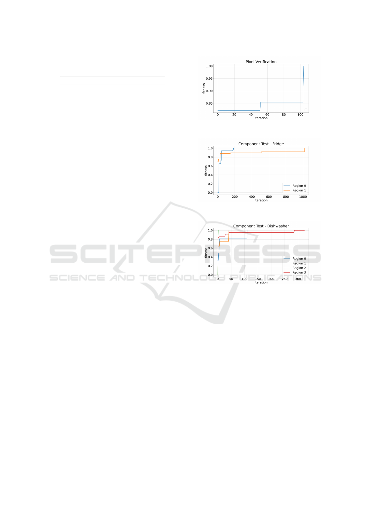
Table 2: Average iterations ±σ until a ﬁtness value of 1 is

reached (rounded to full iterations).

data set region iterations

Pixel veriﬁcation - 86 ± 11

Fridge 0 167 ± 17

Fridge 1 912 ± 83

Dishwasher 0 101 ± 7

Dishwasher 1 38 ± 3

Dishwasher 2 3 ± 1

Dishwasher 3 293 ± 21

6.1 Learning Process

In Figure 3 we display the learning process of our

GA on the three data sets. We decided to visualize

the longest encountered runs as thus we show the ex-

perienced worst case behaviour and additionally give

insight about the encountered ﬁtness function. How-

ever, we also documented the average number of iter-

ations until a ﬁtness value of 1 is reached in Table 2.

We could achieve ﬁtness values of 1 on each test data

set.

Figure 3 (a) shows the results for our oven data set

(pixel veriﬁcation). There we could achieve an op-

timal ﬁtness value rather quickly and we could only

observe three plateaus for the ﬁtness function. The ﬁt-

ness function on the fridge data (Figure 3 (b)) is more

diverse and the GA needs much longer to achieve an

optimal value. Region 1 is harder to learn for the GA

as it contains more icons. We could also observe dif-

fering learning times for the dishwasher data (Figure 3

(c)). Especially regions 2 and 3 are highly different. A

closer look at our data revealed that region 2 is quickly

learned because it only contains two rather distinctive

icons. On the other hand, Region 3 displays connec-

tivity icons. These are rather similar which leads to a

need for a more precise set of parameters.

The averaged results displayed in Table 2 show

that there is a certain amount of variance in the learn-

ing process of most regions. Furthermore, the aver-

age number of iterations until convergence is reached

seems to differ from region to region. This can be ver-

iﬁed using statistical tests. We employed a Friedman

test whose null hypothesis is that the average number

of iterations until a ﬁtness value of 1 is reached is the

same for all regions. We computed a p-value below

0.05 which we regard as signiﬁcant. Thus we reject

the null hypothesis and verify our observation that the

region has an impact on the duration of the learning

process.

(a) Longest encountered learning process for the oven

data set.

(b) Longest encountered learning process for the fridge

data set.

washer data set.

Figure 3: Longest runs of the GA that we encountered dur-

ing all performed experiment repetitions.

6.2 Dealing with Incomplete Data

Due to changes in requirements (Nurmuliani et al.,

2004) and the practice of early testing (Olan, 2003),

we think it cannot be assumed that all icons are known

or implemented when testing starts. Hence we simu-

late that we lack the complete knowledge of all known

icons. We drop a certain number of icons from the

training set but keep them in the test set and evalu-

ate if our calibrated CV methods are still capable of

detecting the test data set correctly.

For these experiments we conﬁne to the fridge

data set as it contained the most icons and it was the

data set where we measured the longest learning pro-

cess. We concentrate on region 1. We drop 1,...,12

icons and observe the ﬁtness values on the test data

set. We repeat this 100 times for each number of icons

to drop.

ICINCO 2021 - 18th International Conference on Informatics in Control, Automation and Robotics

372

Table 4: Averaged runtimes in seconds separated by use case and region.

data average runtime σ ROI size

pixel veriﬁcation 0.0180 0.0080 943 × 186

Fridge 0.0284 0.0019 294 × 69

Fridge 0.0234 0.0019 273 × 65

Dishwasher 0.2186 0.0021 250 × 641

Dishwasher 0.0309 0.0018 204 × 111

Dishwasher 0.0299 0.0026 190 × 117

Dishwasher 0.0117 0.0011 98 × 83

Table 3: Averaged ﬁtness values on the test data set of the

fridge HMI if certain icons are dropped. For the ﬁrst 8 icons

no drop could be detected.

dropped icons average ﬁtness σ

9 0.9827 0.00459

10 0.9783 0.00603

11 0.97810 0.00605

12 0.97482 0.00916

We summarized our results in Table 3. It can be

seen that we can drop up to 8 icons without reduc-

ing the ﬁtness on the test data set. If more icons are

dropped we see a reduction in terms of the ﬁtness.

Hence, a calibration can deal with new icons that were

not available during the training to a certain degree. If

we had used a neural network then we would have had

to adapt the network architecture (the output layer)

and we would have had to retrain it in order to recog-

nize the upcoming GUI elements. With our approach

we need, in the worst case, a retraining but no adapta-

tion of the model. Note that we could observe similar

effects for the other two data sets.

6.3 Runtime Considerations

Testing pursues the goal to ﬁnd errors and ensure

product quality. However, the long-term goal of every

company is to earn money. Therefore testing infras-

tructure should also be viewed from an economical

point of view.

Table 5: Averaged runtimes in seconds for the Raspberry Pi

setting.

average runtime σ ROI size

0.2618 0.0017 92 × 51

0.2065 0.0015 80 × 47

0.2158 0.0019 36 × 40

0.2656 0.0017 80 × 50

0.1980 0.0012 70 × 38

The runtime of a piece of testing infrastructure is

crucial since it is a limiting factor for the number of

tests that can be executed. High runtimes may lead to

more test stands that must be acquired and maintained

which in turn leads to a rise in development cost. Thus

we shortly want to summarize and discuss the ob-

served execution times on our desktop computer.

We measured the runtimes of the pixel veriﬁcation

method using images with a resolution of 943 × 186

pixels. We did the same for Algorithm 2 on the fridge

and dishwasher images which have a resolution of

1490 × 423 and 1399 × 400 respectively.

The averaged results can be seen in Table 4. We

used the combined training and test data sets for the

estimation. Both algorithms have runtimes of less

than one second and, if the regions are rather small,

the execution time may be even less than 100 ms.

7 CONCLUSION AND FUTURE

WORK

We examined two use cases located in the visual ver-

iﬁcation of human machine interfaces (HMI). There

are already commercial solutions available which re-

quire test engineers to choose parameters of com-

puter vision methods such as pixel veriﬁcation man-

ually. We developed a ﬁtness function and employed

a genetic algorithm to automatically ﬁne tune exist-

ing computer vision models. Thus we could erase the

tester engineer’s pain of choosing parameters manu-

ally.

We performed a ﬁrst proof of concept on sev-

eral different industrial data sets. After a reasonable

amount of training we were able to correctly iden-

tify icons and could detect pixel errors. Further, our

designed algorithms have rather low execution times

which enables us to run high numbers of tests.

Furthermore, we veriﬁed our approach on differ-

ent hardware solutions (regarding computer and cam-

era) where we were able to underline the hardware-

independence of our method. This included Rasp-

berry Pi setup which enables companies to cheaply

A Genetic Algorithm for HMI Test Infrastructure Fine Tuning

373

apply our evolutionary technique (if compared to

desktop solutions).

From an engineering perspective we are going to

roll out our system in BSH Home Appliances. Our

next scientiﬁc goal is to employ evolutionary tech-

niques to other computer vision models.

REFERENCES

egroth, E., Feldt, R., and Kolstr

om, P. (2016). Main-

tenance of Automated Test Suites in Industry: An

Empirical study on Visual GUI Testing. CoRR,

abs/1602.01226.

egroth, E., Feldt, R., and Olsson, H. H. (2013). Transi-

tioning Manual System Test Suites to Automated Test-

ing: An Industrial Case Study. In 2013 IEEE Sixth

International Conference on Software Testing, Veriﬁ-

cation and Validation, pages 56–65.

Ammann, P. and Offutt, J. (2016). Introduction to Software

Testing. Cambridge University Press, Cambridge.

Attia, K. A., Nassar, M. W., El-Zeiny, M. B., and Serag,

A. (2017). Fireﬂy Algorithm versus Genetic Algo-

rithm as powerful variable Selection Tools and their

Effect on different multivariate Calibration Models in

Spectroscopy: A comparative Study. Spectrochim-

ica Acta Part A: Molecular and Biomolecular Spec-

troscopy, 170:117 – 123.

Baeza-Yates, R. A. and Ribeiro-Neto, B. (1999). Mod-

ern Information Retrieval. Addison-Wesley Longman

Publishing Co., Inc., USA.

Duan, L., Hofer, A., and Hussmann, H. (2010). Model-

Based Testing of Infotainment Systems on the Basis of

a Graphical Human-Machine Interface. In 2010 Sec-

ond International Conference on Advances in System

Testing and Validation Lifecycle, pages 5–9.

Froglogic (2020). OCR and Installing Tesseract

for Squish. https://doc.froglogic.com/squish/latest/

ins-tessseract-for-squish.html. [Online; accessed 28-

January-2021].

eron, A. (2017). Hands-on machine learning with Scikit-

Learn and TensorFlow : concepts, tools, and tech-

niques to build intelligent systems. O’Reilly Media,

Sebastopol, CA.

Hierons, R. M. (2005). Artiﬁcial Intelligence Methods

In Software Testing. Edited by Mark Last, Abraham

Kandel and Horst Bunke. Published by World Sci-

entiﬁc Publishing, Singapore, Series in Machine Per-

ception and Artiﬁcial Intelligence, Volume 56, 2004.

ISBN: 981-238-854-0. Pp. 208: Book Reviews. Softw.

Test. Verif. Reliab., 15(2):135–136.

Holland, J. H. (1992). Genetic Algorithms. Scientiﬁc Amer-

ican, 267(1):66–73.

Howe, A. E., Mayrhauser, A. V., Mraz, R. T., and Setliff, D.

(1997). Test Case Generation as an AI Planning Prob-

lem. Automated Software Engineering, 4:77–106.

Lara, R. A., Naboni, E., Pernigotto, G., Cappelletti, F.,

Zhang, Y., Barzon, F., Gasparella, A., and Ro-

magnoni, P. (2017). Optimization Tools for Build-

ing Energy Model Calibration. Energy Procedia,

111:1060 – 1069. 8th International Conference on

Sustainability in Energy and Buildings, SEB-16, 11-

13 September 2016, Turin, Italy.

Lowe, D. G. (1999). Object Recognition from Local Scale-

Invariant Features. In Proceedings of the Seventh

IEEE International Conference on Computer Vision,

volume 2, pages 1150–1157 vol.2.

Marwedel, P. (2010). Embedded System Design: Embed-

ded Systems Foundations of Cyber-Physical Systems.

Springer Publishing Company, Incorporated, 2nd edi-

tion.

Mateo Navarro, P., Martinez Perez, G., and Sevilla, D.

(2010). Open HMI-Tester: An open and cross-

platform Architecture for GUI Testing and Certiﬁca-

tion. Computer Systems Science and Engineering,

25:283–296.

Nurmuliani, N., Zowghi, D., and Powell, S. (2004). Anal-

ysis of Requirements Volatility during Software De-

velopment Life Cycle. In 2004 Australian Software

Engineering Conference. Proceedings., pages 28–37.

Olan, M. (2003). Unit Testing: Test Early, Test Often. J.

Comput. Sci. Coll., 19(2):319–328.

OpenCV.org (2020). ORB (Oriented FAST and Rotated

BRIEF). https://opencv-python-tutroals.readthedocs.

io/en/latest/py tutorials/py feature2d/py orb/py orb.

html. [Online; accessed 28-January-2021].

Ramler, R. and Ziebermayr, T. (2017). What You See Is

What You Test - Augmenting Software Testing with

Computer Vision. In 2017 IEEE International Confer-

ence on Software Testing, Veriﬁcation and Validation

Workshops (ICSTW), pages 398–400.

Rauf, A., Jaffar, A., and Shahid, A. (2011). Fully Auto-

mated GUI Testing and Coverage Analysis using Ge-

netic Algorithms. International Journal of Innovative

Computing, Information and Control, 7.

Rublee, E., Rabaud, V., Konolige, K., and Bradski, G.

(2011). ORB: An efﬁcient Alternative to SIFT or

SURF. In 2011 International Conference on Com-

puter Vision, pages 2564–2571.

Singhal, A. (2001). Modern Information Retrieval: A Brief

Overview. IEEE Data Engineering Bulletin, 24.

Stegherr, H., Heider, M., and H

ahner, J. (2020). Classifying

Metaheuristics: Towards a uniﬁed multi-level Classi-

ﬁcation System. Natural Computing.

Szeliski, R. (2010). Computer Vision: Algorithms and Ap-

plications. Springer-Verlag, Berlin, Heidelberg, 1st

edition.

Zeenyx (2020). AscentialTest: Does Im-

age Recognition support some toler-

ance? https://novalys.net/support/index.php?

/atguest/Knowledgebase/Article/View/832/100/

does-image-recognition-support-some-tolerance.

[Online; accessed 28-January-2021].

ICINCO 2021 - 18th International Conference on Informatics in Control, Automation and Robotics

374