Energy Consumption Modeling for Specific Washing Programs of
Horizontal Washing Machine using System Identification
Yongki Yoon
a
and Sibel Malkos¸
b
Washing Machine R&D, Arc¸elik A.S¸., Istanbul, Turkey
Keywords:
Energy Consumption, Energy Efficiency, Data Monitoring, State-space Model, System Identification.
Abstract:
This paper presents the application of an energy consumption modeling technique using a system identification
method regarding the washing program settings for a horizontal washing machine. The observer/Kalman
filter identification/eigensystem realization algorithm (OKID/ERA) method is employed to identify the linear
discrete state-space model by choosing the system order computed by the significant singular values. The
identified model is used as an estimator to figure out the energy consumption level for washing programs with
the full loading condition, and results show the feasibility of the method in energy consumption modeling.
1 INTRODUCTION
The electricity and the water consumption in the
washing machines are mainly dependent on the us-
age pattern of an end-user such as the washing pro-
gram, the temperature setting, the program duration,
the auxiliary functions and the laundry amount as well
as the capacity of the washing machine (Schmitz and
Stamminger, 2014; Afzalan and Jazizadeh, 2019). In
the European Union, horizontal washing machines
are commonly used for the laundry, while vertical
washing machines are mostly populated in the North
America, Asia and Australia. A vertical washing ma-
chine uses more water than a horizontal one, while the
latter consumes more power to control the water tem-
perature via a heater which is a high power consump-
tion device (Pakula and Stamminger, 2010; Bertocco
et al., 2020). In general, researches are mainly fo-
cused on the total energy consumption to provide
the energy-policy direction either in the residential
buildings or in the household appliances. Richardson
(Richardson et al., 2010) presented the annual energy
demand for the household appliances using the statis-
tics between the energy use and the occupant activ-
ity. In references (Bourdeau et al., 2019; Li and Wen,
2014), authors reviewed a data-driven method for the
purpose of the modeling and forecasting in a build-
ing sector and pointed out the popular approaches
such as statistical regression, k-nearest neighbors, de-
a
https://orcid.org/0000-0002-5277-1697
b
https://orcid.org/0000-0002-2159-5766
cision tree, support vector machines, artificial neural-
network, etc. A simplified model of the energy con-
sumption for horizontal washing machines was pro-
posed using a linear relationship regarding the age of
the end-user, the temperature setting, the capacity of
washer and the energy efficiency (Milani et al., 2015).
Recently, a modeling framework was shared by us-
ing a bottom-up activity to estimate the accurate en-
ergy consumption in residential buildings (Leroy and
Yannou, 2018). However, these researches have been
conducted to create the energy model for all types of
household appliances over a year or daily-base to fig-
ure out the optimal energy saving purpose. In house-
hold appliance sector, monitoring the power and the
energy consumption in real-time per unit will give
more flexibility to give the efficient product design
and development strategy.
Addressing the modeling strategy for new product de-
velopment, the system identification methodology is
the most favourable framework by system designers.
For several decades, this method has been an emerg-
ing research topic to characterize the system behavior
using the experimental data to overcome the knowl-
edge gap from the physics-based modeling in the en-
gineering fields (Ljung, 1999; Van Overschee and
De Moor, 1994; Juang and Pappa, 1985). However,
the limited studies were reported in a washing ma-
chine sector using this approach. Therefore we pro-
pose an innovative approach to develop the mathemat-
ical model in a systematic way and the prediction per-
formance of the energy consumption from the mea-
sured data for specific washing programs subjected
Yoon, Y. and Malko¸s, S.
Energy Consumption Modeling for Specific Washing Programs of Horizontal Washing Machine using System Identification.
DOI: 10.5220/0010511407210727
In Proceedings of the 18th International Conference on Informatics in Control, Automation and Robotics (ICINCO 2021), pages 721-727
ISBN: 978-989-758-522-7
Copyright
c
 2021 by SCITEPRESS – Science and Technology Publications, Lda. All rights reserved
721

to the washing program type, the temperature setting,
the drum speed profile, the laundry amount, the un-
balanced load, the amount of detergent and the wa-
ter intake volume (Boyano et al., 2020). The goal of
this research is to develop a framework identifying the
mathematical model from the measured input-output
data sets during the washing cycles and to estimate the
energy consumption without a power sensor in order
to reduce the product cost.
2 PROBLEM STATEMENT
In order to predict and analyze the energy consump-
tion in a washing machine, a mathematical model is
necessary to clarify its characteristics from the mea-
sured data sets. Therefore, an identification process is
required to relate how the input affects the output. In
this research, we consider that a washing machine is
a black-box system for an energy consumption mod-
eling induced by multiple input variables such as a
washing program type (P), a temperature setting (T ),
a profile of motor speed (ω
d
), a laundry amount (m
l
),
an amount of detergent (m
d
), an amount of water
(V ), and so forth in equation (1). In order to address
the multiple inputs and the single output relationship,
we employ an observer/Kalman filter identification
(OKID) working on the time-domain in Figure 1.
E = f (P,T,ω
d
,m
l
,m
d
,V ) (1)
Black-Box
Model
OKID/ERA
u(k) y(k)
u(k)
y(k)
ˆ
A,
ˆ
B,
ˆ
C,
ˆ
D, G
Figure 1: The system identification process.
Taking into consideration of the real application,
we relate the input physical quantities in equation (1)
to the low-level mechanical actuators subjected to a
heater on-time, a pre-wash valve on-time, a main-
wash on-time, a pump on-time, and a profile of motor
speed.
3 DATA AND METHOD
3.1 Data
Firstly, the washing program types were selected
based on widely used programs in the European
Union via Amazon Web Services (AWS) connected
by HomeWhiz IoT ecosystem developed by Arce-
lik. The QUICKWASH and the BEDDING programs
were popularly chosen washing programs by the cus-
tomers, therefore we have collected the input-output
data sets for these washing programs from the same
washing machine with the full load case (9 kg of
etamine fabric) described in Table 1 and the test setup
environment in Figure 2.
Table 1: A washing machine configuration for the test.
Washing Program BEDDING QUICKWASH
Test Condition Load Amount (kg) 9 9
Load Type etamine (70×70cm) etamine (70×70cm)
Spin Speed (rpm) 1000 1400
Temperature (
◦
C) 40 40
Current Total Max. Current (A) 8.4 8.4
Washing Motor Current (A) 0.52 0.6
Spinning Motor Current (A) 2.67 2.5
Power Washing Motor Power (W) 110 86
Total Max. Power (W) 1912 1870
Water Level Main Wash (lt) 21.17 21.10
1. Rinse (lt) 19.44 -
2. Rinse (lt) 19.55 -
Softener (lt) 19.50 21.10
Total Water Consumption (lt) 89.60 43.12
Spin Speed Washing RPM 54 75
Main Wash Spinning RPM 300-617 840
1. Rinse Spin RPM 300-615 -
2. Rinse Spin RPM 300-618 -
Final Spin RPM 300-1020 839
Duration Total Program Duration (min) 110 40
Figure 2: Overview of the test station.
Figures 3-4 show the measured data set regarding
the washing program selection. In the both figures,
during the heater activation to reach the targeted water
temperature (40
◦
C), it consumes most of the energy
between (3-8) minutes and (20 − 22) minutes for the
QUICKWASH program, and between (14-33) min-
utes for the Bedding program. Afterwards, the second
highest energy consumption is caused by the motor
run, and also the amount of water volume in the drum
affects the motor power consumption. Additionally,
the amount of water volume in a washing machine
is determined by the amount of detergent dosage, the
pre-wash valve on-time, the main-wash valve on-time
and the drain pump on-time. Therefore, some of the
inputs are dependent to the others, and this effect will
be simplified via the linear system identification pro-
cess. In this research, a model to be identified is the
multiple-inputs and the single-output (MISO) system
subjected to u ∈ R
5
, y ∈ R
1
. In order to apply the sys-
tem identification, we collected following input and
output data sets as follow.
ICINCO 2021 - 18th International Conference on Informatics in Control, Automation and Robotics
722

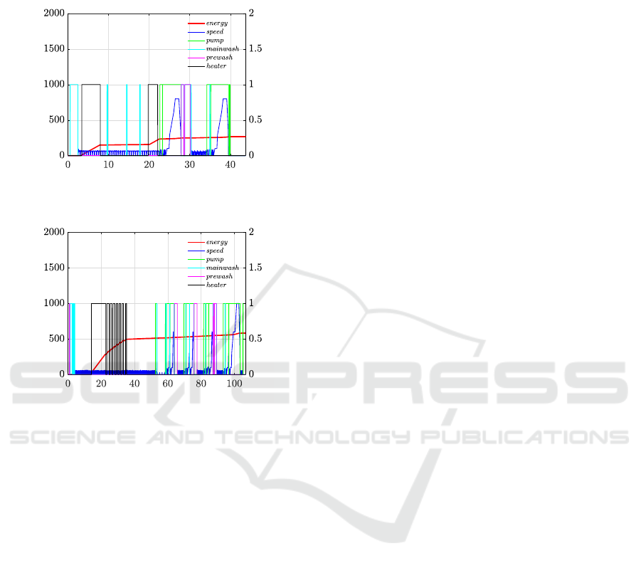
u = [drum speed, heater on-time, prewash valve
on-time, main-wash valve on-time, pump on-time]
y = energy consumption
Time [min]
Energy Consumption / Motor Speed
Valve ON-OFF
Figure 3: Input-output data for the QUICKWASH program.
Time [min]
Energy Consumption / Motor Speed
Valve ON-OFF
Figure 4: Input-output data for the BEDDING program.
3.2 Method
This section reviews the OKID/ERA method (Juang,
1994) to identify the system characteristics using the
input-output data histories of a horizontal washing
machine. Consider a discrete linear time-invariant
system in a state-space form as below,
x(k + 1) = Ax(k) + Bu(k)
y(k) = Cx(k) + Du(k) (2)
where x(k) ∈ R
n
is the system state, y(k) ∈ R
m
is
the output, u(k) ∈ R
r
is the input, and the system ma-
trices are defined as A ∈ R
n×n
, B ∈ R
n×r
, C ∈ R
m×n
,
D ∈ R
m×r
.
By assuming the zero initial condition of the state,
the sequence of the above equations can be written as,
x(k) =
k
∑
i=1
A
i−1
Bu(k − i)
y(k) =
k
∑
i=1
CA
i−1
Bu(k − i) +Du(k) (3)
Then, the output y(k) can be decomposed into the
system Markov parameters (Y ) and the upper triangu-
lar input matrix (U) as below,
y = YU (4)
where y ∈ R
m×l
, Y ∈ R
m×rl
, U ∈ R
rl×l
, and k =
l − 1
From the above equation (4), Y represents the ma-
trix composed of the pulse responses known as the
system Markov parameters to be identified in equa-
tion (5).
Y =

D CB CAB · · · CA
l−2
B

(5)
The upper triangular input matrix is defined as
U =






u(0) u(1) u(2) · ·· u(l − 1)
u(0) u(1) · · · u(l − 2)
u(0) · ·· u(l − 3)
.
.
.
.
.
.
u(0)






and the output vector y is measured as
y =

y(0) y(1) · · · y(2) y(l − 1)

Equation (5) can be directly derived from equation
(2), however, it is not easy to measure the full states of
the system and it does not guarantee the fast compu-
tation and also robust convergence if the data length l
is too large. To solve these issues, the observer gain
matrix G is employed to the state equation (5) to re-
shape the system eigenvalues so that one can obtain
the desired system behavior.
x(k + 1) = Ax(k) + Bu(k) + Gy(k) − Gy(k)
= (A + GC)x(k) + (B +GD)u(k) − Gy(k)
(6)
Then, we can design the new system containing
the observer gain G in the system below,
x(k + 1) =
¯
Ax(k) +
¯
Bv(k) (7)
where
¯
A = A + GC,
¯
B =

B + GD −G

,
v(k) =

u(k) y(k)

T
.
The observer gain matrix G is chosen to make the
system matrix
¯
A to be Hurwitz, and this means that
for some sufficiently large p,
¯
A
k
≈ 0 for time steps k ≥
p. The Kalman filter makes the computation faster to
obtain the observer gain matrix G such that G = −K,
where K is the Kalman gain matrix.
The output equation from the updated system in-
cluding the non-zero initial condition can be written
as
¯y(k) = C
¯
A
k
x(0) +
k
∑
i=1
C
¯
A
k−i
¯
Bv(k − i) +Du(k) (8)
Energy Consumption Modeling for Specific Washing Programs of Horizontal Washing Machine using System Identification
723

Similarly, we can decompose output as below since
the initial condition is negligible due to
¯
A
k
≈ 0
¯y =
¯
Y
¯
V (9)
where ¯y ∈ R
m×(l−p)
,
¯
Y ∈ R
m×[(m+r)p+r]
,
¯
V ∈
R
[(m+r)p+r]×(l− p)
.
Firstly, we compute the observer Markov parame-
ter matrix
¯
Y from equation (10) by taking the pseudo-
inverse.
¯
Y = ¯y
¯
V
†
(10)
where
¯
V
†
=
¯
V
T

¯
V
¯
V
T

−1
¯y =

y(p) y(p + 1) · ·· y(l − 1)

¯
Y =

D C
¯
B C
¯
A
¯
B · ·· C
¯
A
p−1
¯
B

¯
V =






u(p) u(p + 1) · · · u(l − 1)
v(p − 1) v(p) · ·· v(l − 2)
v(p − 2) v(p − 1) · ·· v(l − 3)
.
.
.
.
.
.
.
.
.
.
.
.
v(0) v(1) · ·· v(l − p − 1)






Secondly, the system Markov parameters (Y ) can
be recovered from the observer Markov parameters
(
¯
Y ), and the observer Markov parameters are also ex-
pressed with the system matrices and the observer
gain matrix as below,
¯
Y
0
= D
¯
Y
k
= C
¯
A
k−1
¯
B
=

C (A + GC)
k−1
(B +GD) −C (A + GC)
k−1
G

(11)
or
¯
Y
k
=
h
¯
Y
(1)
k
−
¯
Y
(2)
k
i
(12)
By the induction process, the system Markov pa-
rameters are obtained in equation (13).
Y
0
= D
Y
k
=
¯
Y
(1)
k
−
k
∑
i=1
¯
Y
(2)
i
Y
k−i
f or k = 1, 2,· · · , p
Y
k
= −
p
∑
i=1
¯
Y
(2)
i
Y
k−i
f or k = p + 1, p + 2,∞ (13)
Now, using the eigensystem realization algorithm
proposed by Juang and Pappa (Juang and Pappa,
1985), The Hankel matrix composed of the observer
and the system Markov parameters can be constructed
in equation (14).
H(k −1) =





Y
k
Y
k+1
· · · Y
k+β−1
Y
k+1
Y
k+2
· · · Y
k+β
.
.
.
.
.
.
.
.
.
.
.
.
Y
k+α−1
Y
k+α
· · · Y
k+α+β−2





(14)
The Hankel matrix can be also represented by us-
ing the system Markov parameters in equation (15).
H(k − 1) =




C
C
A
· · ·
CA
β−1




A
k−1
h
B AB · · · A
β−1
B
i
= OA
k−1
C (15)
where C and O denote the controllability and the ob-
servability matrices, respectively. From the Hankel
matrix, a singular value decomposition is performed
to obtain the unitary matrices (U
n
,V
n
) and a singular
value matrix (Σ
n
) for k = 1.
H(0) = U
n
Σ
n
V
T
n
(16)
The singular value matrix (Σ
n
) contains the n number
of singular values whose magnitudes are bigger than
zero such that σ
1
≥ σ
2
≥ · · ·σ
n
> 0. At this stage, one
can check the relative magnitude of the singular val-
ues, and eliminate the values which are not significant
to the system performance (i.e., characteristics), and
determine the system order.
Therefore, the estimated system matrices
(
ˆ
A,
ˆ
B,
ˆ
C,
ˆ
D) can be obtained in equation (17).
ˆ
A = Σ
−1/2
n
U
T
n
H(1)V
n
Σ
−1/2
n
ˆ
B = Σ
1/2
n
V
T
n
E
r
ˆ
C = E
T
m
U
n
Σ
1/2
n
D = Y
0
(17)
where E
T
m
and E
T
r
are consisted of the identity and
the zero matrices, which have different matrix dimen-
sion.
4 RESULTS
The system identification process has been performed
with three measurements for both QUICKWASH and
BEDDING programs from 9 kg capacity of a single
washing machine. Two of the three measurements
have been used to construct the discrete state-space
model using an OKID/ERA method for each wash-
ing program. The third measurement was used for the
validation of the identified model. The data process-
ing, the algorithm implementation, and the simulation
were carried out using MATLAB scripts (MATLAB
R2019a) with Control System Toolbox.
4.1 Model Selection
In general, the singular value represents the charac-
teristics of the system, and it is a reasonable criteria
ICINCO 2021 - 18th International Conference on Informatics in Control, Automation and Robotics
724

Table 2: The identified discrete state-space model.
QUICKWASH BEDDING
ˆ
A



0.8893 0.4491 −0.0631
0.2284 0.1618 −0.5788
−0.1193 0.6037 −0.0331






1.0157 0.2100 −0.0806
−0.1125 0.2362 −0.8358
−0.0155 0.5006 −0.2665



ˆ
B



−0.0005 −0.3207 0.0574 0.0107 0.0243
0.0010 −0.0727 0.0458 −0.0065 −0.0404
−0.0001 0.7456 0.2538 0.0133 −0.0082






−0.0002 −0.3592 0.0031 0.0055 −0.0029
0.0004 −0.2068 0.0043 −0.0020 0.0120
−0.0005 0.6957 −0.0116 0.0113 0.0101



ˆ
C
h
−0.5708 0.3617 0.0367
i h
−0.4659 0.2141 0.0726
i
ˆ
D
h
−0.0002 0.1861 0.0015 −0.0065 −0.0646
i h
0.0001 0.1439 −0.0023 0.0034 0.0010
i
G
h
1.7099 −0.0989 −0.1664
i
T
h
1.5168 −1.0481 −0.7498
i
T
to determine the system size. Therefore, we initially
chose the system size as 10-th order as seen in Fig-
ures 5-6 and the singular values were computed from
the Hankel matrix. Thus, one can choose the system
order by checking the number of the dominant sin-
gular values. In this way, we can reduce the system
order since the rest of the singular values have less
impact to be the system behavior or it can be noise
effects. For the QUICKWASH program in Figure 5,
first three singular values are dominant compared to
the others, and for the BEDDING program, we chose
the first three values since the third and the forth ones
do not have big difference in magnitude. The identi-
fied mathematical models with observers (G) have the
three-degree of freedom described in Table 2.
1 2 3 4 5 6 7 8 9 10
Number of Singular Values
10
-8
10
-7
10
-6
10
-5
10
-4
Magnitude of Singular Values
Figure 5: The singular values for the QUICKWASH.
1 2 3 4 5 6 7 8 9 10
Number of Singular Values
10
-10
10
-9
10
-8
10
-7
10
-6
10
-5
Magnitude of Singular Values
Figure 6: The singular values for the BEDDING.
Both the identified state-space models are control-
lable and observable since we can obtain the full rank
from the controllability and the observability matri-
ces, respectively. Tables 3 and 4 show the accuracy of
the identified model in RMSE and MAPE.
RMSE =
s
1
n
n
∑
i=1
( ˆy
i
− y
i
)
2
(18)
MAPE =
1
n
n
∑
i=1




ˆy
i
− y
i
y
i




(19)
Table 3: Model accuracy for the QUICKWASH program.
Observer Test No. E
rmse
(Wh) E
mape
(%)
Test 1 0.1467 7.71 × 10
−4
Yes Test 2 0.1407 7.67 × 10
−4
Test 1 13.9991 6.6575
No Test 2 12.5445 5.9351
Table 4: Model accuracy for the BEDDING program.
Observer Test No. E
rmse
(Wh) E
mape
(%)
Test 1 0.1331 1.48 × 10
−4
Yes Test 2 0.1291 2.00 × 10
−4
Test 1 10.2693 1.9780
No Test 2 10.2693 1.978
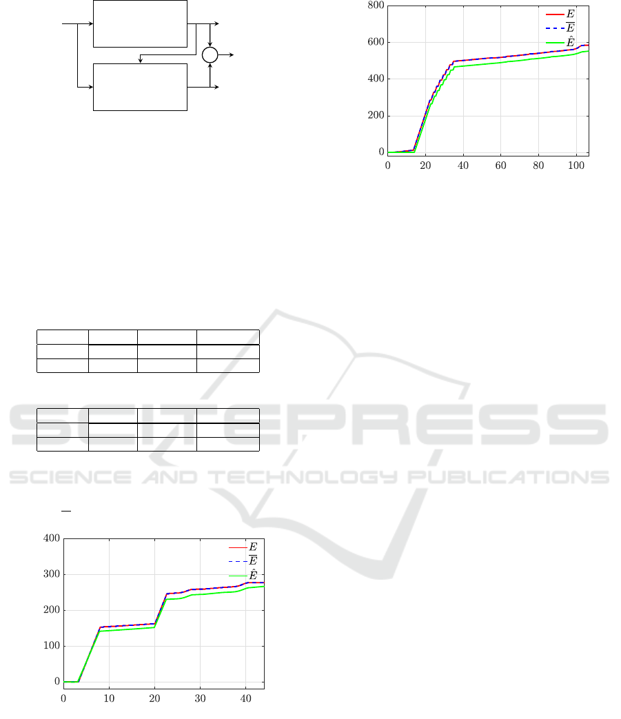
4.2 Model Validation
From the identified state-space model in Table 2, we
used the third measurement data, which was not in-
cluded for the system identification process, to vali-
date the prediction accuracy of the energy consump-
tion for both washing programs in Figure 7. Tables
5 and 6 indicate the errors in the RMSE and the
MAPE defined in equations (18)-(19). Both tables
show that adding an observer (G) provides the ac-
curate energy estimation since the augmented input,
v(k) =

u(k) y(k)

T
in equation (7), contains the
input measurement as well as the output via sensors.
That means the observer generates the optimal system
states by minimizing the error between the measured
energy consumption and the estimated one.
In Figure 7, the estimated output is defined by ˆy
k
at
each time step and the errors are calculated as below,
Energy Consumption Modeling for Specific Washing Programs of Horizontal Washing Machine using System Identification
725

Washing Machine
Identified Model
(
ˆ
A,
ˆ
B,
ˆ
C,
ˆ
D, G)
u
k
y
k
ˆy
k
+
−
e
k
Figure 7: The model validation.
In this research, however, we focused on identify-
ing the linear discrete state-space model and validat-
ing the accuracy of the model by comparing the pre-
dicted output to the measured one. The results show
that the identified MISO model without an observer
roughly follows the trend of the energy consumption
with the accuracy of 91.2% and 94.2% in MAPE for
the QUICKWASH and the BEDDING programs, re-
spectively.
Table 5: Validation for the QUICKWASH program.
Observer Test No. E
rmse
(Wh) E
mape
(%)
Yes Test 3 0.1435 7.48 × 10
−4
No Test 3 18.1276 8.8069
Table 6: Validation for the BEDDING program.
Observer Test No. E
rmse
(Wh) E
mape
(%)
Yes Test 3 0.1575 8.19 × 10
−5
No Test 3 28.0675 5.8599
Figures 8-9 also graphically demonstrate that how
well the model with and without an observer estimates
the energy consumption, where
ˆ
E is without an ob-
server and E with an observer.
Time [min]
Energy Consumption [Wh]
Figure 8: Comparison of the energy consumption for the
QUICKWASH program.
Time [min]
Energy Consumption [Wh]
Figure 9: Comparison of the energy consumption for the
BEDDING program.
5 CONCLUSION AND FUTURE
WORK
In this research, we have studied the systematic mod-
eling technique for the energy consumption in a hor-
izontal washing machine using an OKID/ERA ap-
proach in the time-domain and the model reduction
process was carried out to reduce the computational
time by counting the dominant singular values ob-
tained from the Hankel matrix. The discrete lin-
ear time-invariant state-space models with the three-
degree of freedom were obtained and validated to see
the feasibility of the framework for the energy con-
sumption of the specific washing programs. From the
simulation results, the method can successfully gen-
erate the accurate model with the input-output mea-
surements. Especially, in the case of being used as
an estimator with Kalman gain (K = −G) in a feed-
back system to adjust the optimal system states, the
prediction accuracy in the energy consumption can be
significantly improved. For the future study, we will
consider medium and large capacity of washing ma-
chines under the different laundry amounts such as
quarter, half and full loading. The proposed model
will be integrated and deployed in the software stack
of washing machine to estimate the energy consump-
tion level without a power sensor to check the practi-
cal aspect.
REFERENCES
Afzalan, M. and Jazizadeh, F. (2019). Residential loads
flexibility potential for demand response using energy
consumption patterns and user segments. Applied En-
ergy, 254:113693.
Bertocco, M., De Dominicis, M., Favaro, I., Ferri, A.,
Ronchi, F., Salmaso, L., Spadoni, L., and Stellini, M.
ICINCO 2021 - 18th International Conference on Informatics in Control, Automation and Robotics
726

(2020). Impact of limestone incrustation on energy
efficiency of washing machine. Energy Efficiency,
13(1):1–15.
Bourdeau, M., qiang Zhai, X., Nefzaoui, E., Guo, X.,
and Chatellier, P. (2019). Modeling and forecast-
ing building energy consumption: A review of data-
driven techniques. Sustainable Cities and Society,
48:101533.
Boyano, A., Espinosa, N., and Villanueva, A. (2020).
Rescaling the energy label for washing machines: an
opportunity to bring technology development and con-
sumer behaviour closer together. Energy Efficiency,
13(1):51–67.
Juang, J.-N. (1994). Applied system identification. Prentice-
Hall, Inc.
Juang, J.-N. and Pappa, R. S. (1985). An eigensystem re-
alization algorithm for modal parameter identification
and model reduction. Journal of guidance, control,
and dynamics, 8(5):620–627.
Leroy, Y. and Yannou, B. (2018). An activity-based mod-
elling framework for quantifying occupants’ energy
consumption in residential buildings. Computers in
Industry, 103:1–13.
Li, X. and Wen, J. (2014). Building energy consumption
on-line forecasting using physics based system identi-
fication. Energy and buildings, 82:1–12.
Ljung, L. (1999). System identification. Wiley encyclopedia
of electrical and electronics engineering, pages 1–19.
Milani, A., Camarda, C., and Savoldi, L. (2015). A sim-
plified model for the electrical energy consumption of
washing machines. Journal of Building Engineering,
2:69–76.
Pakula, C. and Stamminger, R. (2010). Electricity and wa-
ter consumption for laundry washing by washing ma-
chine worldwide. Energy efficiency, 3(4):365–382.
Richardson, I., Thomson, M., Infield, D., and Clifford,
C. (2010). Domestic electricity use: A high-
resolution energy demand model. Energy and build-
ings, 42(10):1878–1887.
Schmitz, A. and Stamminger, R. (2014). Usage behaviour
and related energy consumption of european con-
sumers for washing and drying. Energy Efficiency,
7(6):937–954.
Van Overschee, P. and De Moor, B. (1994). N4sid:
Subspace algorithms for the identification of com-
bined deterministic-stochastic systems. Automatica,
30(1):75–93.
Energy Consumption Modeling for Specific Washing Programs of Horizontal Washing Machine using System Identification
727