Optimization-based or AI Task Planning
for Scenarios with Cooperating Mobile Manipulators?
Stefan-Octavian Bezrucav, Yifan Liu and Burkhard Corves
Institute of Mechanism Theory, Machine Dynamics and Robotics,
RWTH Aachen University, Eilfschornsteinstrasse 18, 52062 Aachen, Germany
Keywords:
Task Planning, Mobile Manipulators, MILP, CP, Temporal AI Planning.
Abstract:
Task planning has become one of the most important components of the control system for teams of coop-
erating robotic systems in complex scenarios. It plays such a critical role, as it must determine, order and
assign a high variety of different tasks to the involved actors, such that at the end, the goals are reached while
some metric, as the total execution time, is minimized. In this paper the analysis of three task planning ap-
proaches, mixed-integer linear programming (MILP), constraint programming (CP) and automated temporal
planning (TP), with respect to three criteria is targeted. These criteria are the CPU time for plan generation,
the plan makespan and the flexibility of the modelling approach. For the analysis, an intricate scenario in a
kitchen environment with a team of multiple mobile manipulators is developed. The models and results are
then compared to derive the advantages and disadvantages of each strategy.
1 INTRODUCTION
With the increasing complexity of automation scenar-
ios it is necessary that more actors cooperate in order
to reach more elaborate goals. These complex goals
imply that the actors must not execute anymore only
a small, fixed set of repetitive actions. They need
to perform intricate tasks that must be selected and
scheduled based on their capabilities and considering
interactions, the actual status of the system and the
goals. In these cases, the process of determining the
sequence of tasks needed to be executed and their as-
signment to the actors is not anymore trivial. This
process is called task planning and it becomes even
more challenging when some optimization goals, like
a minimal total execution time, are thrived.
This paper is part of a bigger work in which six
different planning strategies for automation scenar-
ios with cooperating mobile manipulators are stud-
ied. They are Mixed-Integer Linear Programming,
Constraint Programming, Temporal Planning, Auc-
tion Algorithms, Genetic Algorithms and Hierarchi-
cal Task Network. In the followings, the focus is
set only on the first three approaches. The usability
of these approaches is analysed by evaluating them
with respect to three factors: the model flexibility
(the effort required to adapt the model for a differ-
ent planning problem of the same scenario), the plan
makespan (total execution time) and the CPU time to
generate that plan. For this purpose, a special scenario
with mobile manipulators in a kitchen environment is
designed to present the different possibilities to model
and solve task planning problems.
2 BACKGROUND
In this paper, three different planning strategies are
studied. Mixed-Integer Linear Programming (MILP)
and Constraint Programming (CP) are two mathemat-
ical optimization approaches. MILP tackles prob-
lems which contains a series of variables (continuous
or integer), parameters, linear constraints and a lin-
ear objective function to be optimized. The standard
technique to solve MILP problems is represented by
branch-and-bound algorithms (Land, A. H. and Doig,
A. G., 1960). The idea of this method is to iteratively
partition the feasible solution region into more subdi-
visions (nodes) and ignore the integer-requirements
to acquire a linear program (LP) in each subdivi-
sion. The LP at each node in the search tree is then
solved with the Simplex method, which returns a set
of boundaries that are used to guide the solving pro-
cess (Murty, 1985). Task planning problems can be
then formulated as MILP problems and solved with
the above algorithms. For example, in (Booth et al.,
2016) and (Yi et al., 2020), MILP is applied for multi-
robot task planning problems in a retirement home
and in a kitchen scenario.
Bezrucav, S., Liu, Y. and Corves, B.
Optimization-based or AI Task Planning for Scenarios with Cooperating Mobile Manipulators?.
DOI: 10.5220/0010509001150122
In Proceedings of the 18th International Conference on Informatics in Control, Automation and Robotics (ICINCO 2021), pages 115-122
ISBN: 978-989-758-522-7
Copyright
c
 2021 by SCITEPRESS – Science and Technology Publications, Lda. All rights reserved
115

CP is more general than MILP, as it can solve
problems with various types of variables and con-
straints in a wide range of arithmetic expressions
(Gervet, 2006). The solving process, called Con-
straint Propagation, is also a tree search. Different to
MILP, instead of solving a LP-program, at each node
the values set of a variable is reduced by eliminat-
ing those values that violate the problem constraints
(Rossi et al., 2006). Like MILP, CP is also used
in many industrial applications, such as assignment
problems (Simonis, 2001) and scheduling problems
(Behrens, J. K. et al., 2019) and (Mokhtarzadeh, M.
et al., 2020). In (Booth et al., 2016) and (Ku, W.-Y.,
Beck, J. C., 2016), CP is applied to solve the same
task planning and job shop scheduling problems, as
MILP does, in order to make a comparison between
them.
The last planning strategy, Temporal Planning
(TP), is an AI planning technique. The planning prob-
lem is usually described through a domain in which
the types of the elements from the environment, the
predicates and the possible actions are defined. The
predicates are boolean functions which can take one
or more previously defined types, as variables. Each
state of the environment is described through a set
of grounded predicates, which represent the boolean
functions that are true for specific input values. For
example, the predicate agv at pose ?agv ?pose can be
grounded to agv at pose agv1 pose2, which implies
that agv1 is at pose pose2. At the end, the actions are
used to modify the values of the predicates and thus
transform one state in another one. Given an initial
state described by a set of grounded predicates, the
TP algorithms search and order with specific heuris-
tics the grounded actions that must be executed such
that the system is transformed from the given state to a
state in which all set goals are achieved. The planning
problem is encoded in the Plannin Domain Defini-
tion Language (PDDL) (Fox and Long, 2003) that can
be understood by different automated planners. One
widely used deterministic heuristic temporal planner
is POPF (Coles et al., 2010). Such approaches were
used for example in (Bezrucav and Corves, 2020).
3 MODEL AND CONCEPT
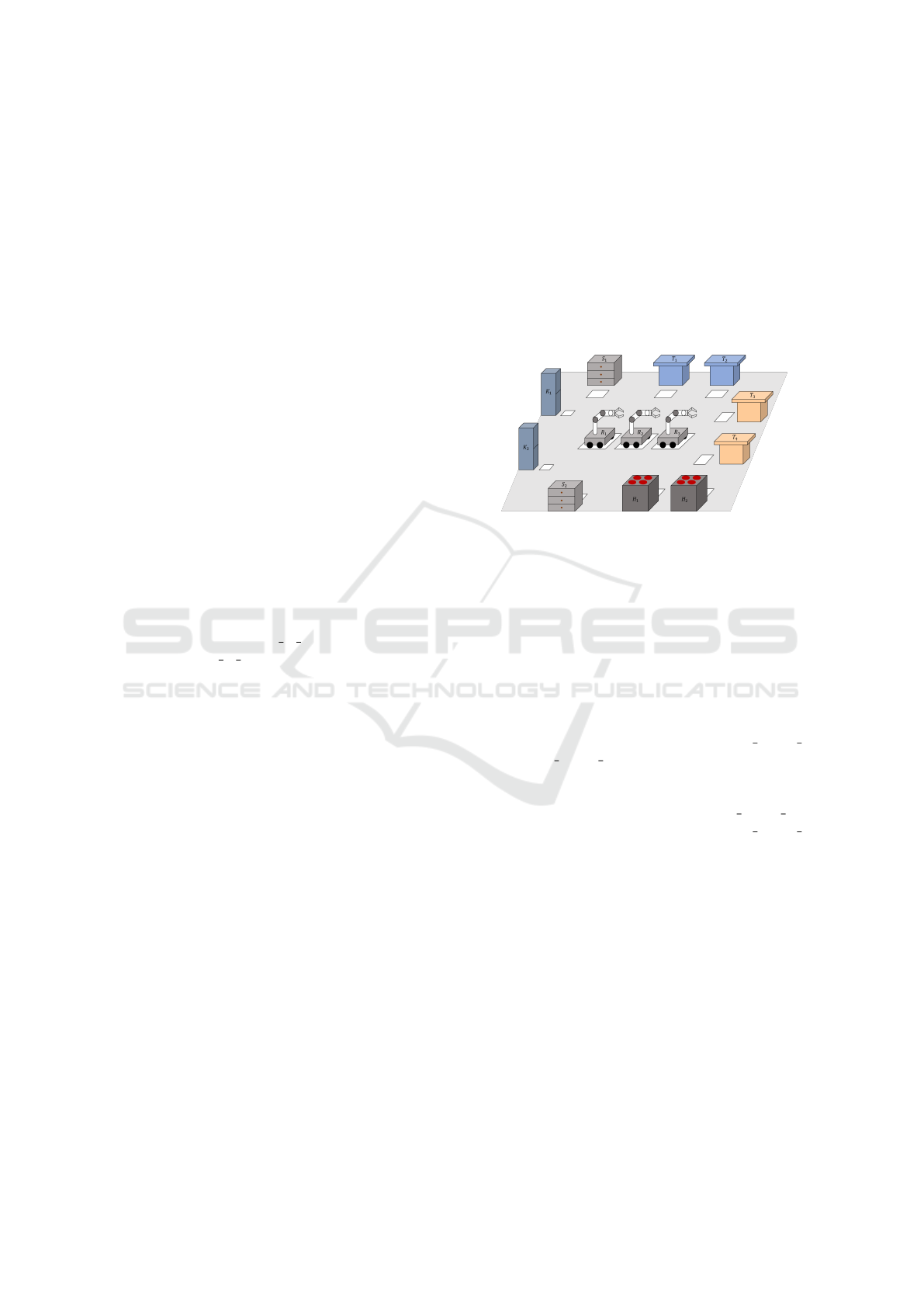
In this paper, a scenario in the kitchen of a restaurant
is defined, in which a team of mobile manipulators
executes a series of specific tasks in this shared space.
The scenario consists of two parts, the physical world
and the planning problem. The physical world can be
further divided into the environment and the mobile
manipulators, both of which are shown in Figure 1.
The environment contains two tool-banks, two refrig-
erators, two cookers, two worktables and two normal
tables. The refrigerators K
1
, K
2
store all the neces-
sary food required to cook meals and the tool-benches
S
1
, S
2
offer the necessary tools for the cooking pro-
cess. The worktables T
1
, T
2
and cookers H
1
, H
2
pro-
vide the places to process the food. On the right side,
there are two normal tables T
3
, T
4
where robots can
put the finished food on. There is only one fixed park-
ing pose near to all locations (white squares), where
the mobile manipulators can park.
Figure 1: The kitchen scenario with mobile manipulators.
The planning problem includes the initial state of
the system, the goals, the available actions and fur-
ther rules that must be obeyed. In the initial state, all
pasta are kept in portions in refrigerator K
1
and all sal-
ads in refrigerator K
2
. The tools to process the salad
and pasta are stored in tool-banks S
1
and S
2
. At the
beginning, the robots are parked on the initial posi-
tions shown in Figure 1. There are two kinds of goals
in this framework: processing the salad and cooking
the pasta. The actions that the robots can execute are
move, load, unload, attach, detach, generic action 1
and generic action 2. The execution duration of all
actions except for the move action are fixed. The exe-
cution duration of the latter represents the travel time
between the different locations. generic action 1 is
the action to process the salad and generic action 2
implies cooking the pasta. The generic actions must
be executed with the corresponding tools and food
portions and at the selected positions. The salad must
be processed on worktable T
1
or T
2
and pasta should
be cooked on the cooker H
1
or H
2
. After the pasta or
salad is well processed, the salad must be served on
the table T
3
and the pasta on T
4
. Moreover, the robots
should also bring the tools back to the corresponding
tool-banks at the end.
A task precedence graph for one goal to process
the salad and two goals to cook the pasta is shown
in Figure 2. The actions required in order to reach
these two types of goals and their precedence are de-
tailed with the help of this precedence graph. In order
to process the salad (T1 - T7), any of the robots must
travel to the refrigerator K
1
, load the salad, then move
ICINCO 2021 - 18th International Conference on Informatics in Control, Automation and Robotics
116

Figure 2: The task precedence graph for the planning prob-
lem.
to the worktable T
1
or T
2
and unload the salad. Be-
sides, the same robot, or another one, should go to the
tool-bank S
1
and attach the tool. The load action (T1)
must be executed before the unload action (T3), but
there is no precedence constraint between the attach
action (T2) and the load, unload actions (T1, T3). Af-
ter T1, T2 and T3 are finished, generic action 1 (T4)
can be carried out in order to make the salad. Then,
the finished salad must be loaded from worktable (T5)
and be taken to table T
3
as well as unload it (T6). At
last, the tool should be detached at tool-bank S
1
(T7).
Analogously, the only precedence constraint between
tasks T5, T6 and T7 is that T5 should be finished
before T6 starts. Additionally, all the tasks can be
done cooperatively, by different mobile manipulators,
as long as the constraints are all fulfilled. The second
and third goals, to cook the pasta, can be reached with
a similar pattern (T8 - T14 and T15- T21 in Figure 2).
In order to make the task planning problems for
this scenario closer to real-world problems, some gen-
eral rules are also made and formulated as constraints:
1. Each robot can take up to two portions of food at
a time.
2. Each robot can have up to one tool at a time.
3. Each location in the environment can be visited
by only one robot at a time.
4. Precedence rule: The fixed task precedence rules
in Figure 2 must be obeyed.
5. Same-robot rule: Some tasks must always be fin-
ished by the same robot.
6. Same-place rule: Some tasks must always be fin-
ished at the same places.
While the first three rules are straight-forward, the
fourth rule is important especially when tasks that are
related in one precedence order are allocated to differ-
ent robots, e.g. T3 is assigned to robot R1 and T4 to
R2. This is a known as a cross-schedule dependency.
Table 1: Task planning problems with G goals and R robots.
R G goal types
Pb. 1 3 3 (salad, pasta, pasta)
Pb. 2 2 3 (salad, pasta, pasta)
In this case, the two tasks are separated in two sched-
ules, therefore, the schedules of these robots should
be carefully managed, so that the tasks are executed
in the correct order. Apart from the precedence con-
straints, those tasks from Figure 2 are also not com-
pletely independent one from another. Some tasks
must be finished by the same robot, such as T1 and
T3, because the robot who loads the food to its plat-
form should also unload it. The working places of
some tasks should be the same like T3 and T4, be-
cause generic action 1 should be executed where the
food is unloaded. Hence, the last two rules are also
included.
Due to the high-complexity of the model that con-
siders that many interactions and constraints for the
actors and tasks, only planning problems with a low
number of robots and goals are solvable. In this con-
text, only two task planning problems in the kitchen
scenario for R robots and G goals are considered.
Their parametrization is presented in Table 1.
4 MODELLING AND RESULTS
This section includes the description of the models
and the plans generated with the MILP, CP and Tem-
poral planning approaches.
4.1 MILP and CP
The same model can be used for both the MILP and
CP strategies. It is defined as:
Parameters:
N : set of tasks, N = {1, 2,..., J}
M : set of robots, M = {1, 2, ..., R}
O : sets of possible positions for each task
O = {1 : [..], .., J : [..]}
p
i j
: coord. of position j for task i, ∀i ∈ N, j ∈ O[i]
a
i
: coord. of the initial position of robot i, ∀i ∈ M
t
i
: time consumption of task i, ∀i ∈ N
H : a large integer, such as 100000
P : set of task pairs who should obey
the precedence rule
S : set of task pairs who should obey
the same-robot rule
Optimization-based or AI Task Planning for Scenarios with Cooperating Mobile Manipulators?
117

W : set of task pairs who should obey
the same-place rule
T : set of ”attach” and ”detach” task pairs
F : set of ”load” and ”unload” task pairs
Variables:
x
i j
=
(
1 if task i is assigned to robot j
0 otherwise, ∀i ∈ N, j ∈ M
z
in
=
(
1 if task i is executed at position n
0 otherwise, ∀i ∈ N, n ∈ O[i]
y
ik j
=
(
1 if task k is after task i in robot j’s plan
0 otherwise, ∀i, k ∈ N, j ∈ M
q
inkm
=









1 if task k is after task i and both tasks
are executed at the same position
0 otherwise,∀i, k ∈ N, i 6= k, n ∈ O[i],
m ∈ O[k], p
in
= p
km
s
i
: start time of task i, ∀i ∈ N
t
max
: total execution time of the plan
Constraints:
1.
∑
j∈M
x
i j
= 1 ∀i ∈ N
2.
∑
n∈O[i]
z
in
= 1 ∀i ∈ N
3. s
i
+t
i
+ |p
in
− p
km
| ≤ s
k
+ H ∗ ((1 −y
ik j
) + (1−
x
i j
) + (1 − x
k j
) + (1 − z
in
) + (1 − z
km
))
s
k
+t
k
+ |p
in
− p
km
| ≤ s
i
+ H ∗ (y
ik j
+ (1 − x
i j
)
+ (1 − x
k j
) + (1 − z
in
) + (1 − z
km
))
∀i, k ∈ N, i 6= k, n ∈ O[i], m ∈ O[k], j ∈ M
4. s
i
+t
i
≤ s
k
+ H ∗ ((1 −q
inkm
) + (1 − z
in
) + (1−
z
km
))
s
k
+t
k
≤ s
i
+ H ∗ (q
inkm
+ (1 − z
in
) + (1 − z
km
))
∀i, k ∈ N, i 6= k, n ∈ O[i], m ∈ O[k], p
in
= p
km
,
5. y
ik j
= 0 ∀i, k ∈ N, i = k, j ∈ M
6. y
ik j
+ H ∗ (x
il
− 1) ≤ 0, y
ik j
+ H ∗ (x
kl
− 1) ≤ 0,
∀ j, l ∈ M, j 6= l, ∀i, k ∈ N
7. s
i
≥ |a
j
− p
in
| − H ∗ ((1 − x
i j
) +
∑
k∈N
y
ki j
+
(1 − z
in
)), ∀i ∈ N, j ∈ M, n ∈ O[i]
8. s
i
+t
i
+ |p
in
− p
km
| ≤ s
k
+ H ∗ ((1 −z
in
)
+ (1 − z
km
))∀(i, k) ∈ P, n ∈ O[i], m ∈ O[k]
9. x
i j
= x
k j
∀(i, k) ∈ S, j ∈ M
10. z
in
= z
kn
∀(i, k) ∈ W, n ∈ O[i] or O[k]
11. y
a
1
a
2
j
+ y
a
1
b
2
j
+ y
b
1
a
2
j
+ y
b
1
b
2
j
< 4
∀(a, b) ∈ T, ∀ j ∈ M
12. y
a
1
a
2
j
+ y
a
1
b
2
j
+ y
a
1
c
2
j
+ y
b
1
a
2
j
+ y
b
1
b
2
j
+ y
b
1
c
2
j
+ y
c
1
a
2
j
+ y
c
1
b
2
j
+ y
c
1
c
2
j
< 9
∀a, b, c ∈ F, a 6= b, b 6= c, a 6= c, ∀ j ∈ M
13. t
max
≥ s
i
+t
i
∀i ∈ N
Objective function: min t
max
The model consists of four parts. In the parameter
part, two sets of integer numbers N, M are used to
represent all tasks and robots, respectively. In both
problems, J, the total number of tasks, is equal to
21 and R, the total number of robots, is 2 or 3. Fur-
thermore, some tasks have multiple possible locations
where they can be executed, hence, a set O is added
to provide the list of all possible locations where each
task can be executed. For each pair of a task i and a
position j where it can be executed, the coordinate of
that position is defined as p
i j
. Further on, the initial
location of robot i is fixed with the position parameter
a
i
. By setting the positions of each task, the initial and
end conditions, such as the initial and end positions of
the objects from the environment (e.g. the tools and
the foods) are defined. Further on, the sets of task
pairs P, S,W, T, F are defined. A part of the task pairs
corresponding to the precedence graph are presented
in Table 2.
Table 2: Task pairs in parameters P, S,W, T, F.
Parameter Task pairs
P (1,3), (2,4), (3,4), (4,5), (4,7), (5,6)...
S (1,3), (2,4), (4,7), (5,6)...
W (3,4), (4,5)...
T (2,7); (9,14);...
F (1,3), (5,6); (8,10), (12,13)...
Six variables are defined in this model. x
i j
and z
in
are binary decision variables that present the decision
of task and position assignment, respectively. x
i j
is
assigned a value of 1 if task i is allocated to robot j
and 0 otherwise. z
in
has a value of 1, if the position n
is chosen as the location of task i.
Further on, y
ik j
and q
inkm
are both binary decision
variables for task sequence. y
ik j
has the value 1 if
two tasks i and k are assigned to the same robot j and
task i precedes task k. On the other hand, q
inkm
has
a value of 1, if both tasks i and k are executed at the
same place, thus p
in
= p
km
, and task i precedes task k.
Moreover, s
i
presents the start time of task i and t
max
is the total duration of the schedule.
The constraints are defined by the equalities and
inequalities 1-13. The constraints 1 and 2 ensure that
each task is assigned to a robot and each task has
exactly one location where it can be executed. Af-
ter that, the constraint 3 contains two sets of equa-
tions, which are disjunctive sequence constraints to
ICINCO 2021 - 18th International Conference on Informatics in Control, Automation and Robotics
118

prevent the time intervals of the tasks in each robot’s
schedule from overlapping. Both equations take real
effect when the term multiplied with H is equal to
0. For the first equation, this happens when tasks i
and k are executed at position n and m respectively
(1 −z
in
= 1 − z
km
= 0), tasks i and k are both assigned
to robot j (1 − x
i j
= 1 − x
k j
= 0) and task i precedes
k (1 − y
ik j
= 0). The entire inequality then turns to
s
i
+t
i
+|p
in
− p
km
| ≤ s
k
. With the travel time between
two tasks calculated as |p
in
− p
km
| (each robot’s speed
is fixed to 1[-]/s), the inequality forces the start time
of task k to be greater than the finish time of task i
plus the travel time between the poses for tasks i and
k. Otherwise if task i should be after k, thus y
ik j
= 0,
the second equation will take similar effect.
However, if two tasks are planned at the identical
location, their time intervals should also not overlap
even when they might not be assigned to the same
robot (general rule 3). Therefore, constraint 4 is set
up. In case that tasks i and k are executed at loca-
tions n and m and their positions are same (p
in
= p
km
),
if task i precedes k (q
inkm
= 1) the first equation be-
comes s
i
+t
i
≤ s
k
and constrains the start time of task
k and vice versa.
So far, constraint 3 over y
ik j
is defined for the case
that i 6= k and there is no constraint over y
ik j
when
i = k, so constraint 5 is added to constrain y
ik j
for
this case. Besides, the two inequalities in 3 take real
effects only when task i, k are both assigned to robot
j (x
i j
= x
k j
= 1), but there is also no restriction on
the value of y
ik j
, when task i or k is not assigned to
robot j. Hence, constraint 6 is defined. In 6, if task i
is assigned to another robot l instead of j (x
il
= 1) the
inequality turns to y
ik j
≤ 0 and y
ik j
can only be 0 in
such case. When task k is allocated to another robot,
the second equation takes similar effect.
Inequality 7 is developed to constrain the start
time of the first task in each robot’s schedule. If
x
k j
= 1 and
∑
k∈N
y
ki j
= 0, no task precedes task i in
robot j’s schedule, thus, the start time s
i
should be
larger than the travel time between initial position j
and the location of task i (|a
j
− p
in
|).
Constraints 8-12 are developed to make the model
generate plans that obey the general rules from Sec-
tion 3. Constraint 8 is valid for all task pairs in P to
ensure the fixed precedence orders in Figure 2. Con-
straint 9 and 10 make sure that each task pair in S is
allocated to the same robot and each task pair in W is
executed at the same place. These constraints corre-
spond to the general rules 4, 5 and 6. Constraints 11
and 12 aim at limiting the number of tools and food
on each robot respectively (general rule 1 and 2). The
last constraint ensures that the variable t
max
is equal to
or greater than the finish time of any task. At last, the
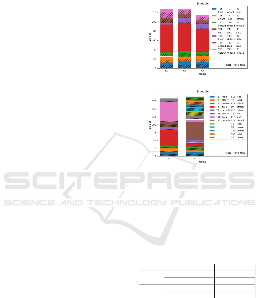
(a) CP result Problem 1.
(b) CP result Problem 2.
Figure 3: The generated plans for both problems using CP.
objective is to minimize t
max
.
In order to compare both strategies, both MILP-
and CP-model are implemented in Python and the
problem is solved with the MILP-solver and CP-
solver in the same optimization software Google OR-
Tools (Da Col and Teppan, 2019). The generated
plans using CP are shown in Figure 3. The makespan
(total execution time) of the solution plans and the
computational efforts are presented in Table 3.
Table 3: MILP and CP solution data for Pb. 1 and Pb. 2.
Method Properties Pb. 1 Pb. 2
MILP
schedule length [s] 128 189
CPU time [s] 49429 3540
CP
schedule length [s] 128 189
CPU time [s] 5.6 4.5
The total length of the plans generated by MILP
and CP are identical, although the task sequence and
allocation are different. The reason behind this is that
both methods stop when they find one of the possible
multiple optimal solutions. An optimal solution still
can include idle time slots that appear due to the gen-
eral constraints of the model (e.g. cross-schedule con-
straints). The high quality of the plans is also shown
in Figure 3. The pauses between tasks are reduced as
Optimization-based or AI Task Planning for Scenarios with Cooperating Mobile Manipulators?
119

Figure 4: The examples of objects that belong to types
”robotpose, foodpose, toolpose”.
much as possible and the tasks are allocated to differ-
ent robots appropriately, so that the total length of the
schedules is minimized.
However, there is an important difference between
the computational time using both strategies. The
MILP-solver needs about 13h and 1h to solve the
problems, while the CP-solver only 5.6s and 4.5s.
This striking contrast is due to different optimization
principles and the property of the problem that most
variables are binary variables. During the search pro-
cess, at each node, CP uses propagation to remove un-
necessary values from the domain of variables. This
strategy is especially efficient when dealing with bi-
nary variables, as their domain is only {0, 1} and the
propagation engine only needs to check quite a small
number of values in each iteration. As in our model
nearly 99% of variables are binary variables, CP man-
ages to solve the problem very fast. Nevertheless,
this advantage is not exploited by the MILP solver,
as MILP solves an integer linear program to get the
optimum at each node. Therefore, the optimization
strategy of MILP ignores the advantage of binary vari-
ables’ small domain and treats them as normal contin-
uous variables.
4.2 Temporal Planning
In this section, the temporal planning (TP) model
written in PDDL and the plans generated for it with
the POPF planner are presented and discussed.
This model consists of two parts: the domain and
the problem model. The domain model can be further
split into types, predicates, functions and actions.
As shown in Listing 1 four basic types of ob-
jects and three different types of positions (Figure 4)
are defined (lines 2-3). Robotposes are places where
robots can stand on (white squares). Tools and food
can be put on toolposes and foodposes, respectively,
and these types are defined to set limitations on the
number of tools and food items that can be held at
a time. In the predicates-part (lines 4-11), the first
predicates describe the state of different objects and
the following ones are used to determine whether the
correct position, tool and food are chosen for each
generic action. The function move cost is used to cal-
culate the travel time.
Listing 1: Excerpt from the PDDL domain file.
1 ( : t y p e s
2 robo t food t o o l p o si t io n - ob j e ct
3 r o bo t po s e fo o dp o se t o o l p o s e - ←-
po s it i on )
4 ( : p r e d i c a t e s
5 ( at ? o 1 -o b j e ct ? o 2- o bj e c t )
6 ( free ? p os e- p o s i t i o n )
7 ( n ot _ a c ti n g ? r ob o t - r o bo t )
8 ( u n c o ok e d ? f-foo d ) ( co ok e d ? f -f o o d )
9 ( f o o d_ fo r _ g a _ 1 ? f - f oo d )
10 ( t o o l_ fo r _ f o o d ? t - t oo l ? f - fo o d )
11 ( p o s _f o r _ g a _ 1 ? p - r o b ot p o s e ) . . .
12 ( : f u n c t i o n s
13 ( m ov e _c o s t ? f r o m ? to - r o bo t p o se ) )
14
15 ( : d u r a t i v e − a c t i o n move
16 : p a r a m e t e r s
17 ( ? r - robot ? from ? to - robo t p o se )
18 : d u r a t i o n
19 ( = ? d ur a ti o n ( mov e _c o st ? f r o m ? to ) )
20 : c o n d i t i o n
21 ( at star t ( ( at ? r ? fr om ) ( fr e e ? to )
22 ( n ot _ a c ti n g ? r ) )
23 : e f f e c t
24 ( at star t ( ( n o t ( at ? r ? from ) )
25 ( n o t ( not_ a c t in g ? r ) )
26 ( n o t ( f r e e ? to ) ) ) )
27 ( at e n d ( ( a t ? r ? t o ) ( not _ a c ti n g ? r )
28 ( f r e e ? f r o m ) ) ) )
29 . . .
Further on, in the domain file seven actions
are defined: move, load, unload, attach, detach,
generic action 1, generic action 2, corresponding to
the actions that robots can execute. The setting for the
move action is also shown in Listing 1, in lines 16-28.
Its duration is calculated with the function move cost.
According to the defined conditions, it can only be
executed when robot r is at start position f rom, in an
idle state, and the goal place to is free. The effect in
”at start” means that all predicates at, not acting, f ree
are removed immediately after the action execution is
started. At the end of this action, the state is modified
such that robot r is at the target position to, in an idle
state, and the start place f rom is free. The other ac-
tions are defined similarly, but due to space issues are
not presented here.
In the problem-model the objects, the initial state
and the goal state of the planning instance are defined
as depicted in Listing 2. Using the types from the
domain, f ood, tool and robot objects are declared
(lines 2-4). Further on, for each robot and for each
location a fixed number of robotposes, foodposes and
toolposes are set (lines 5-7). The initial state is set
up with grounded predicates. In lines 9-10, it is de-
fined that all robots are not executing any task and
that all the food is uncooked. In lines 11-13, the ini-
ICINCO 2021 - 18th International Conference on Informatics in Control, Automation and Robotics
120

tial positions for the robots, the tools and the food are
fixed. After that, in lines 14-15, the foodposes and
toolposes are connected to the corresponding robots
or robotposes. All these positions should be free at
first. The locations, food items and tools required
for both generic actions are specified in lines 16-17
and in line 18 all move costs are set. In the goal state
the cooked meals must be placed on tables T
3
and the
tools must be returned to the tool-banks S
1
(lines 21-
23). At last, the objective is set to minimize the total
time (line 24).
Listing 2: The objects, the initial state, the goal state and
the metric in the problem file.
1 ( : o b j e c t s
2 food 1 foo d 2 fo o d 3 - f ood
3 tool 1 too l 2 to o l 3 - t ool
4 ro b o t1 rob o t 2 r ob o t 3 - ro b ot
5 r o bo t 1 _ fp 1 . . . - f o od p o s e
6 r o bo t 1 _ tp 1 . . . - t o ol p o s e
7 co o ke r 1 . . . - r o b o tp o se . . . )
8 ( : i n i t
9 ( n ot _ a c ti n g rob o t1 ) . . .
10 ( u n c o ok e d f o od1 ) . . .
11 ( at rob o t 1 in i t i a l _ p o s e1 ) . . .
12 ( at food 1 r e f r i g e r a t o r 1 _f p1 ) . . .
13 ( at tool 1 t o o l b a nk 1_ t p 1 ) . . .
14 ( at ro b o t 1_ f p 1 r o bot 1 )
15 ( free r o b o t 1 _ fp 1 ) . . .
16 ( p o s _f o r _ g a _ 1 wt1 )
17 ( f o o d_ fo r _ g a _ 1 food 1 ) . . .
18 ( t o o l_ fo r _ f o o d tool 1 foo d 1 ) . . .
19 ( = ( mo v e _c o st c o o ke r 1 wt1 ) 8 ) . . .
20 ( : g o a l
21 ( ( at f o o d1 ta b le 3_ f p1 ) . . .
22 ( at tool 1 t o o l b a nk 1_ t p 1 ) . . .
23 ( c o oke d fo o d 1 ) . . . ) )
24 ( : m e t r i c m in im i ze ( tot a l- t i m e ) )
The main feature of this modelling approach is its
high flexibility. The model only provides the initial
and end state without offering a clear guidance of
the intermediate steps of achieving the goal. This
increases the difficulty of solving the problem, but
makes the approach much more flexible. The gener-
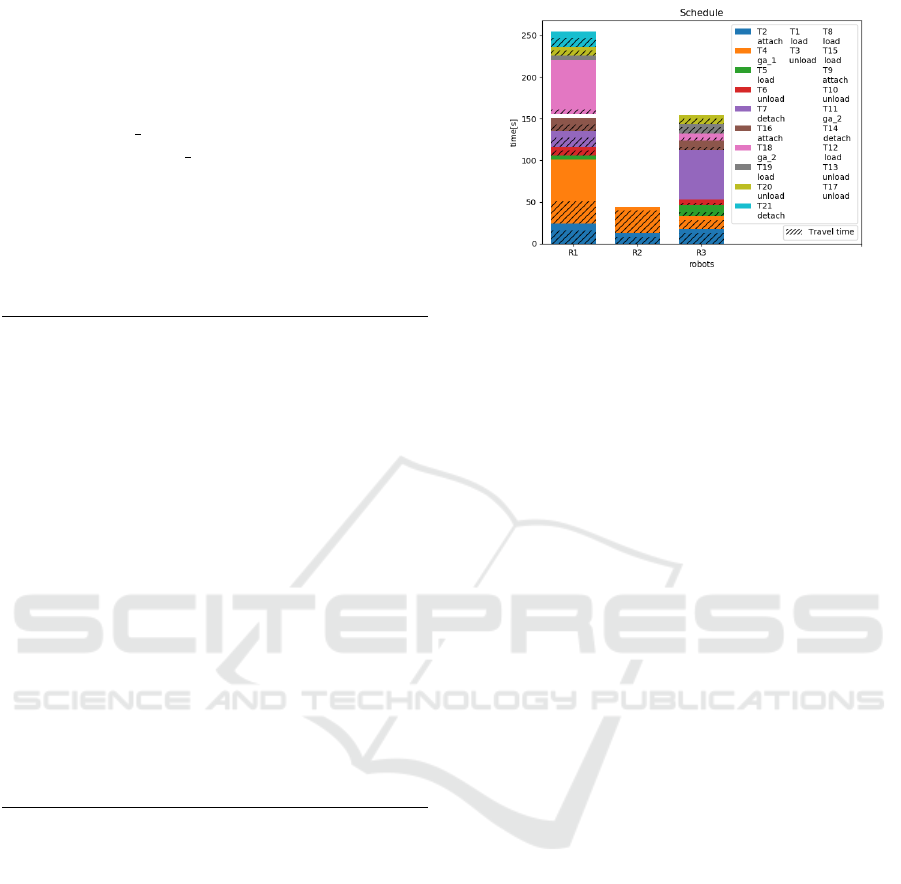
ated plan for the first problem is shown in Figure 5.
Its total lengths of 255s can be explained by the large
proportion of time spent on travelling. The second
drawback is that the tasks are not allocated properly.
Only two tasks are assigned to robot R
2
, who could
take more tasks from R
1
to reduce the total working
time. There are two possible reasons for the bad plan
quality. Firstly, the heuristic in the planner POPF
could be the cause. Similar issues are also reported in
the paper introducing POPF (Coles et al., 2010). Sec-
ondly, as mentioned above, offering no clear guidance
of the intermediate steps to achieve the goal makes the
Figure 5: Problem 1, makespan: 255s.
number of possible states in the search space
large and that increases the difficulty to solve the
problems.
4.3 Comparison and Discussions
In this section, the three strategies are compared from
three perspectives: model flexibility, CPU time and
makespan.
The model flexibility referred here relates to the
effort required to adapt the model for a different plan-
ning problem of the same scenario. This is a crucial
factor, because there may be various types of plan-
ning problems in a real-world scenario. In order to
evaluate the flexibility, a new planning problem based
on the old one from Figure 2 is defined: the salad
no longer needs to be processed and can be put di-
rectly on table T
3
or T
4
. Starting with the CP and
MILP model, the parameters and the sets P, S,W, T, F
must be changed by hand, as the number of tasks is
reduced and some task pairs from the problem’s sets
are removed. Furthermore, the indices of all parame-
ters and the precedence graph must also be modified.
On the other hand, for the TP model only the initial
state in the problem-part needs to be modified: cooked
food1 is updated to uncooked food1. This modifi-
cation is quite simple comparing to that of CP and
MILP model. The reason behind this is that the math-
ematical model is based on the task precedence graph,
which substantially provides a clear direction of how
to solve the problem. Therefore, when the require-
ments of the problem change, the direction and all
inputs related to it have to be modified. In contrast,
the TP model offers little limitation and guidance on
intermediate steps in the process of moving from the
initial state to the end state. Hence, the change of in-
termediate steps can be ignored and only the initial-
and goal state need to be adapted. In conclusion, the
MILP and CP models are evaluated with low flexibil-
ity and TP model has very high flexibility.
Optimization-based or AI Task Planning for Scenarios with Cooperating Mobile Manipulators?
121

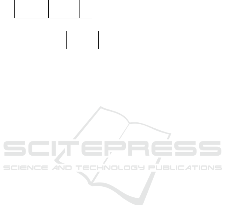
Table 4: CPU time of runs using each strategy.
CP MILP TP
CPU Pb. 1 [s] 5.6 49429 47
CPU Pb. 2 [s] 4.5 3540 3.2
Table 5: Makespan of plans generated with each strategy.
CP MILP TP
Makespan Pb. 1 [s] 128 128 255
Makespan Pb. 2 [s] 189 189 306
The second factor is the CPU time, which is de-
picted for all problems and all planning approaches in
Table 4. All computations were done on a computer
with Intel
R

Core
TM
i5-6200U CPU at 2.30 GHz and 8
GB of RAM. For both problems, CP shows great and
stable performance regarding the CPU time, whereas
MILP is almost impractical. The computational time
with TP is even lower than that with CP for prob-
lem 2, but is also relatively high for problem 1. This
means that when the number of objects in the model
increases, the CPU time with TP also grows rapidly.
Hence, CP is the best choice among these three strate-
gies with respect to the CPU time. Considering the
makespans of the generated plans, as depicted in Ta-
ble 5, CP and MILP are both highly efficient, while
TP shows bad performance.
Moreover, for each strategy multiple ways to de-
velop a model are possible and different models may
lead to different results. This is the case for the TP ap-
proach, where the quality of the plan highly depends
on the matching between the used heuristic and the
model of the planning problem. However, if different
CP or MILP based models are applied for the same
problem, the CPU time may be different, but the gen-
erated plan is always the global optimal solution re-
garding makespan.
5 CONCLUSIONS
In this work the modelling and solving of a complex
task planning problem with three planning strategies
is presented. CP shows the greatest performance in
terms of CPU time and plan quality (makespan of
plans), while temporal planning is the best when con-
sidering the flexibility of the models. In the next steps,
we aim to solve the model with further MILP, CP and
TP planners. A further direction for our future work is
to combine the CP and TP approaches to complement
each other and thus being able to improve the overall
performance on all three factors.
REFERENCES
Behrens, J. K., Lange, R., and Mansouri, M. (2019). A con-
straint programming approach to simultaneous task
allocation and motion scheduling for industrial dual-
arm manipulation tasks. In 2019 International Con-
ference on Robotics and Automation (ICRA). IEEE.
Bezrucav, S.-O. and Corves, B. (2020). Improved ai plan-
ning for cooperating teams of humans and robots. In
Cashmore, M., Orlandini, A., and Finzi, A., editors,
Workshop on Planning and Robotics (PlanRob) at In-
ternational Conference on Automated Planning.
Booth, K. E. C., Tran, T. T., Nejat, G., and Beck, J. C.
(Jan. 2016). Mixed-integer and constraint program-
ming techniques for mobile robot task planning. IEEE
Robotics and Automation Letters, 1(1):500–507.
Coles, A., Coles, A., Fox, M., and Long, D. (2010).
Forward-chaining partial-order planning. In Proceed-
ings of the Twentieth International Conference on
Automated Planning and Scheduling, pages 42–49.
AAAI Press.
Da Col, G. and Teppan, E. (2019). Google vs ibm: A con-
straint solving challenge on the job-shop scheduling
problem. Electronic Proceedings in Theoretical Com-
puter Science, 306:259–265.
Fox, M. and Long, D. (2003). pddl2.1 : An extension to
pddl for expressing temporal planning domains. Jour-
nal Of Artificial Intelligence Research, 20:61–124.
Gervet, C. (2006). Constraints over structured domains. In
Francesca Rossi Peter van Beek Toby Walsh, editor,
Handbook of Constraint Programming, Foundations
of Artificial Intelligence, pages 605–638. Elsevier.
Ku, W.-Y., Beck, J. C. (2016). Mixed integer program-
ming models for job shop scheduling: A computa-
tional analysis. Computers & Operations Research,
73:165–173.
Land, A. H. and Doig, A. G. (1960). An automatic method
of solving discrete programming problems. Econo-
metrica, 28:497–520.
Mokhtarzadeh, M., Tavakkoli-Moghaddam, R., Vahedi-
Nouri, B., and Farsi, A. (2020). Scheduling of
human-robot collaboration in assembly of printed cir-
cuit boards: a constraint programming approach. In-
ternational Journal of Computer Integrated Manufac-
turing, 33(5):460–473.
Murty, K. G. (1985). Linear and Combinatorial Program-
ming. R.E. Krieger.
Rossi, F., Peter van Beek, and Walsh, T., editors (2006).
Handbook of Constraint Programming: Introduction.
Elsevier Science.
Simonis, H. (2001). Building industrial applications with
constraint programming. In Comon, H., Treinen,
R., and March
´
e, C., editors, Constraints in compu-
tational logics: theory and applications, pages 271–
309. Springer-Verlag Berlin Heidelberg, France.
Yi, J.-s., Ahn, M. S., Chae, H., Nam, H., Noh, D., Hong,
D., and Moon, H. (2020). Task planning with mixed-
integer programming for multiple cooking task using
dual-arm robot. In 17th International Conference on
Ubiquitous Robots (UR), pages 29–35. IEEE.
ICINCO 2021 - 18th International Conference on Informatics in Control, Automation and Robotics
122