Bayesian Mixture Estimation without Tears

arka Jozov

1,2 a

, Ev

zenie Uglickich

2 b

and Ivan Nagy

2 c

Faculty of Transportation Sciences, Czech Technical University, Na Florenci 25, 11000 Prague, Czech Republic

Department of Signal Processing, The Czech Academy of Sciences, Institute of Information Theory and Automation,

Pod vod

arenskou v

ı 4, 18208 Prague, Czech Republic

Keywords:

Data Analysis, Clustering, Classiﬁcation, Mixture Model, Estimation, Prior Knowledge.

Abstract:

This paper aims at presenting the on-line non-iterative form of Bayesian mixture estimation. The model used

is composed of a set of sub-models (components) and an estimated pointer variable that currently indicates

the active component. The estimation is built on an approximated Bayes rule using weighted measured data.

The weights are derived from the so called proximity of measured data entries to individual components. The

basis for the generation of the weights are integrated likelihood functions with the inserted point estimates of

the component parameters. One of the main advantages of the presented data analysis method is a possibility

of a simple incorporation of the available prior knowledge. Simple examples with a programming code as

well as results of experiments with real data are demonstrated. The main goal of this paper is to provide

clear description of the Bayesian estimation method based on the approximated likelihood functions, called

proximities.

1 INTRODUCTION

Modeling is an important part of data analysis. It can

be said that there are two main directions the data

analysis aims at. The ﬁrst one looks for the on-line

prediction of data based on the already measured his-

torical ones. Usually, the output variable is to be

predicted depending on its older values and other ex-

planatory variables which can be currently measured.

A dynamic model, e.g., of a regression type, must be

constructed and mostly also estimated in an on-line

way. Here, the task is to determine the value of the

output in a future time instant.

The second data analysis direction is interested in

working modes of a system rather than in the values of

the data themselves. In this direction, classes of sim-

ilar data are constructed and the newly coming data

records are classiﬁed to them, i.e., a class to which

the data record belongs is estimated. The question

here can be, for example, what severity of a trafﬁc ac-

cident we can expect if the surrounding circumstances

are like those just measured.

There are well known methods which can do these

tasks. The most famous methods for clustering are

https://orcid.org/0000-0001-5065-633X

https://orcid.org/0000-0003-1764-5924

https://orcid.org/0000-0002-7847-1932

e.g., k-means and its variants (Jin and Han, 2011;

Kanungo et al., 2002; Likas et al., 2003), fuzzy

clustering (De Oliveira and Pedrycz, 2007; Panda

et al., 2012), DBSCAN (Kumar and Reddy, 2016)

and hierarchical clustering (Nielsen, 2016; Ward Jr,

1963). For classiﬁcation, one can use e.g., neural

networks, decision trees, logistic regression (Mai-

mon and Rokach, 2005; Kaufman and Rousseeuw,

1990) or genetic algorithms (Pernkopf and Bouchaf-

fra, 2005). However, all the mentioned tasks can

be also solved using estimation of a mixture model.

Its iterative version called the EM algorithm (Bilmes,

1998) is also well known.

In this area, methods of mixture estimation based

on the Bayesian principles play an important role.

One of them, called Quasi-Bayes, has been devel-

oped in (K

arn

y et al., 1998) followed by (K

arn

y et al.,

2006). Following this research, several other methods

have been suggested, mostly for different models of

the components exploited (Nagy et al., 2011; Nagy

and Suzdaleva, 2013; Nagy et al., 2017; Suzdaleva

et al., 2017; Suzdaleva and Nagy, 2019), etc. They

bring a considerable simpliﬁcation of the estimating

algorithm. The core of the last of them is the use of

the proximity of the measured data record to a distri-

bution (the model of a speciﬁc working point of the

analyzed system).

Jozová, Š., Uglickich, E. and Nagy, I.

Bayesian Mixture Estimation without Tears.

DOI: 10.5220/0010508706410648

In Proceedings of the 18th International Conference on Informatics in Control, Automation and Robotics (ICINCO 2021), pages 641-648

ISBN: 978-989-758-522-7

641

This paper tries to explain the nature and the func-

tionality of the proximity introduced in (Nagy et al.,

2016; Nagy and Suzdaleva, 2017) as simply as pos-

sible. It also presents the simplest possible form of

the whole mixture estimation algorithm, based on the

proximity, with the hope it will be fully understood

even in its program form.

The paper is organized as follows. The ﬁrst part

is devoted to the link between the density function

of a random variable and its realizations. Here, it is

stressed that in the same way as realizations lie near

the top of the density function, it is possible to say that

the nearer the realization lies to the top of the density

function, the higher is the probability that it belongs

to its random variable. Then the notion of the proxim-

ity and its properties are discussed. The second part

of the paper demonstrates a simple algorithm of mix-

ture estimation in the whole. Conclusions close the

paper.

2 PRELIMINARIES

2.1 Density Function and Its

Realizations

Let us have a scalar normally distributed random vari-

able y with the known expectation µ and variance

r = 1

f (y|µ). (1)

Now, let us generate values y

,··· from this distri-

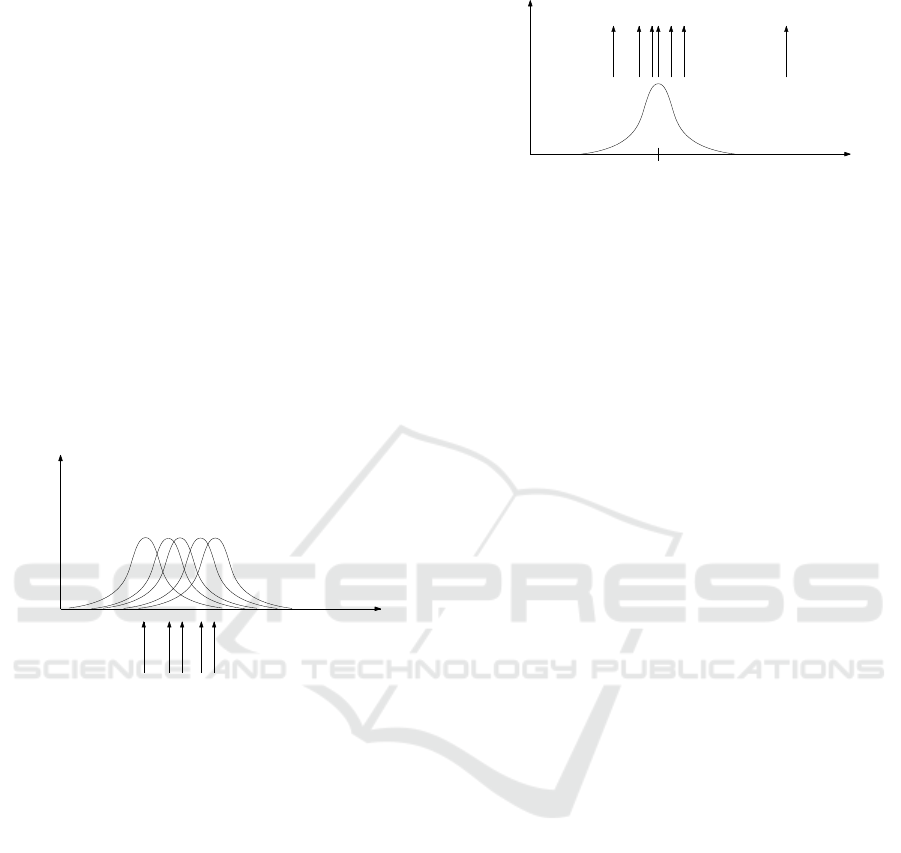
bution. An example of such situation is depicted in

Figure 1. Here we can see the normal distribution and

f(y)

f(y|µ)

Figure 1: A ﬁxed distribution of random variable y with its

realizations.

several values generated from it (the up arrows). Ac-

cording to the nature of the stochastic principles, the

densest are the values near to the top of the density

function. The larger is their distance from the top, the

smaller is the probability of generating such a value.

In Figure 1, the value y

is in a position where the

occurrence of the values is rare and the value y

so far that we can suppose that it has been generated

from some other density function whose expectation

lies somewhere to the right of our one.

The same can be said about measured values. If

the value is near the top of the density estimated from

the past data, we can assume it belongs to it. The more

remote is the value position from the density, the less

is the probability that it belongs to it. If it is very far

from it, we can conclude that it belongs to another

probability density. If in Figure 1 the data y

up to y

have been used for estimation of the depicted density

function, then we can assume y

to come from some

other distribution.

2.2 Likelihood

Likelihood is the most important and frequently used

tool for estimation. It is also a part of the posterior

density produced by the application of the Bayes rule,

see, e.g., (K

arn

y et al., 1998; K

arn

y et al., 2006).

For a model f (y|Θ) with the parameters Θ and the

measured dataset D =

{

,· ·· ,y

}

, the likelihood

(Θ) is deﬁned as a function of Θ and data D with

independent samples

(Θ) =

∏

τ=1

f (y

|Θ), (2)

in the theory of estimation taken as a function of Θ.

However, it can be interpreted also as a function of

actual data y

. We can write

(Θ,y

) ∝

∏

τ=1

f (y

|Θ) = f (y

|Θ)

t−1

∏

τ=1

f (y

|Θ), (3)

where now y

is taken as still unmeasured data en-

try and the rest of values

{

,· ·· ,y

t−1

}

as already

measured and

L denotes the modiﬁed view of the like-

lihood.

If we take an integral of

L over all possible values

of Θ, denoted by Θ

∗

, we obtain

∗

f (y

|Θ)

t−1

∏

τ=1

f (y

|Θ)dΘ = f (y

t−1

t−2

,· ·· ,y

(4)

which is the predictive probability density function of

the actual data y

Thus, we can state:

• L

(Θ) serves for the estimation of the parameter

Θ (the likelihood) and

•

∗

(Θ)dΘ is the predictive density function for

the modeled variable y (the integrated likelihood)

arn

y et al., 2006).

ICINCO 2021 - 18th International Conference on Informatics in Control, Automation and Robotics

642

2.2.1 Use of Likelihood for Parameter

Estimation

We can show the sense of the likelihood as an esti-

mator of the unknown parameter with the help of the

following example.

Let us have a scalar normal random variable y

with the probability density function (denoted by

pdf) f (y|Θ) with the known variance r = 1 and un-

known expectation Θ = µ. For the measured data

{

,· ·· ,y

}

, we can draw the distributions in-

volved in the likelihood as functions of parameters in

Figure 2. As it is known and can be guessed from the

ﬁgure, their product gives a distribution, which lies in

the position of the average value taken as the point es-

timate for this case. Moreover, due to the properties

of the distribution, the product will be a very narrow

function, and the more narrow it is, the more data are

involved. So, the precision of the estimate grows with

the increasing number of data.

f(y)

Figure 2: The product of the distributions involved in the

likelihood.

2.2.2 Use of Likelihood for Prediction

The integrated likelihood taken as a function of the

actual data value y

is the prediction which can be

taken as a measure of the closeness of a measured

value to the predictive density function based on the

model from which the likelihood has been produced.

This is demonstrated in Figure 3.

Figure 3 is similar to Figure 1, but instead of a

ﬁxed distribution, now, we have the estimated predic-

tive one generating the data as predictions. Similarly

to Figure 1, we can see that the distance of a realiza-

tion from the distribution can be viewed as a measure

of membership of the realization to the distribution.

Notice, that the membership is not crisp, but it is

expressed in a form of values of probabilistic weights

(after normalization).

f(y

t−1

, y

t−2

, · · · , y

)

t−1

Figure 3: The distribution of normal random variable in a

role of predictor.

2.3 Proximity

The proximity is deﬁned as the integrated likelihood

arn

y et al., 2006) with the inserted value of the ac-

tual data record y

and actual point estimates of the

parameters

t−1

. It measures a kind of a distance of

from the estimated predictive pdf, which character-

izes the model of y

. In other words, we can say that

the proximity measures the distance of the measured

data entry to the model of the output variable y

. We

can demonstrate its derivation as follows.

As we have said, the integrated likelihood (predic-

tive pdf) has the form

f (y

t−1

t−2

,· ·· ,y

) =

∗

f (y

|Θ)

t−1

∏

τ=1

f (y

|Θ)dΘ,

(5)

where f (y

|Θ) is the model and

∏

t−1

τ=1

f (y

|Θ) is the

likelihood L

t−1

(Θ) for “past” data up to time t − 1.

Using the Maximum Likelihood Estimate (MLE), the

point estimate

t−1

of Θ is the argument of maximum

of the likelihood. Moreover, it is known that for a

sufﬁcient amount of informative data it is a very slim

function. To avoid problems with the integration, we

replace the likelihood by a Dirac function

t−1

(Θ) → δ



Θ −

t−1



, (6)

where δ (x − a) is nonzero only for x = a and accord-

ing to (Temple, 1955)

∞

−∞

δ (a −b)da = 1. (7)

For this function it holds (Kanwal,1998)

∞

−∞

f (x)δ(x − a) dx = f (a) . (8)

Now, when we substitute Dirac function δ



Θ −

t−1



for the likelihood in (5), we obtain the formula for the

proximity q

∗

f (y

|Θ)δ



Θ −

t−1



dΘ = f



t−1



(9)

Its properties fully follow from the above considera-

tions.

Note, the old data are hidden in the estimate

t−1

Bayesian Mixture Estimation without Tears

643

3 BAYESIAN VIEW OF MIXTURE

ESTIMATION

Mixture models (Bouguila and Fan, 2020; McNi-

cholas, 2020; Nagy et al., 2011; Nagy and Suzdal-

eva, 2017) are used for a description of multimodal

data, i.e., data produced by a system that exists in

several working points. Each working point has its

own model called the component and a model that de-

scribes switching of these components.

3.1 Model

A mixture model with static components consists of:

1. A set of ordinary models (components)

|Θ

), i = 1,2,··· , n

with y

the modeled variable and Θ

the param-

eter of the i-th component. They can be arbitrary

models for which a recursive estimation of param-

eters exists, which are mostly models from the ex-

ponential family. Here, we will assume them to

be static Gaussian models in the m-dimensional

space (here, m will be equal to one).

2. A pointer model, which is a categorical model for

a discrete variable called the pointer (K

arn

y et al.,

1998). The pointer value at time t indicates the ac-

tive component, which generates the current data.

The pointer model has the form

f (c

|α) = α

, (10)

where c

denotes the pointer variable at time t and

the parameter α is a vector of probabilities such

that α

≥ 0 ∀i and

∑

i=1

= 1.

3.2 Estimation of the Component

Parameters

There are two different views on how the mixture

models work:

1. The switching of the components is known or the

components are not overlapping, so that we can

measure the switching.

2. The switching is not known and has to be esti-

mated on the basis of data coming from the indi-

vidual working modes that are overlapping, which

makes the estimation unambiguous. All of the

components can be active at the same time, each

with its own probability.

The ﬁrst case is simple and easy to deal with. Each

time instant, knowing exactly the active component,

we fully update its statistics and compute the point

estimates of its model parameters. All other compo-

nents stay unchanged.

3.2.1 Example

For static normal components f

|µ

) with the

known variance and scalar modeled variable, the pa-

rameter µ is the expectation. It is well known, that

the optimal estimate of the expectation is the sample

average that is deﬁned as a sum of measured outputs

divided by their number. That is why we can choose

the statistics as follows: S

, which is the sum of mea-

sured outputs and n

, which is their number. Each

component will have these two statistics. Their on-

line update can be written in the following form

= S

;t−1

+ y

, (11)

= n

;t−1

+ 1, (12)

where c

is the measured (known) label of the active

component at time t.

The second case is more complicated, but also

much more realistic in applications. The basic prob-

lem in this case is the estimation of the weights w

determining the probabilities of the membership of

the measured data item y

to individual components.

These weights are practically given by the normalized

proximities of y

to the currently estimated compo-

nents.

Remarks.

1. Actually, the weights are given not only by prox-

imities, but the proximities are decisive and can

be taken as the only factor for the construction of

the weights.

2. For determining proximities, we need the param-

eter point estimates (see (9)). It means that what

we perform is the point estimation.

From the theoretical derivation it follows that the es-

timation of the individual components is similar to

that for single models (11)–(12). The only differ-

ence is that the statistics of all the components are up-

dated and the actual data added to these statistics are

weighted by the corresponding entry of the weighting

vector w

3.2.2 Example

For the situation introduced in the previous example,

the update of the component statistics can be derived

similarly to (K

arn

y et al., 1998; K

arn

y et al., 2006) as

follows:

i;t

= S

i;t−1

+ w

i;t

, (13)

i;t

= n

i;t−1

+ w

i;t

(14)

for all i = 1, 2,· ·· ,n

. A a result, the measured data

go to each component with the ratio corresponding to

the probability they belong to it.

ICINCO 2021 - 18th International Conference on Informatics in Control, Automation and Robotics

644

Remark. In addition to the estimation of compo-

nents, the pointer model should also be estimated, see

arn

y et al., 1998; K

arn

y et al., 2006). However, its

importance is negligible and the whole pointer model

estimation can be omitted.

3.3 Algorithm of Mixture Estimation

The algorithm of the mixture estimation takes the fol-

lowing form:

Initialization:

1. Set the number of components n

2. Set the initial components f

|Θ

), i =

1,2, ·· · ,n

. Here, they are scalar static Gaussian

models with the known variance and initial

expectation

= ˆµ

3. Set the initial statistics for the component estima-

tion corresponding to the initial parameters. Here,

denotes the vector of the initial sums of the

prior values of y

in the individual components

and n

is the vector of the corresponding initial

numbers of prior data. They can be set according

to the expert knowledge.

Time loop:

For t = 1, 2,··· ,N

1. Measure the current data y

2. Construct the weighting vector w

(a) Compute the proximities q

= f





(b) Normalize the proximities

= [q

,· ·· ,q

∑

i=1

. (15)

3. Perform the update of the component statistics

i;t

= S

i;t−1

+ w

i;t

, (16)

i;t

= n

i;t−1

+ w

i;t

. (17)

4. Compute the point estimates of the expectations

ˆµ

i;t

. (18)

5. For the case of classiﬁcation, determine the actual

component

ˆc

= argmax (w

). (19)

end

3.4 Program for Estimation of Normal

Static Components

A code of the mixture estimation algorithm imple-

mented in a programming free and open source envi-

ronment Scilab (www.scilab.org) is presented below.

// Estimation of a simple mixture

// ------------------------------

clc, clear, close, mode(0)

N=500;

pS=[.5 .2 .3];

mS=[2 5 7];

// Simulation

for t=1:N

cS(t)=sum(rand(1,1,’u’)>cumsum(pS))+1;

y(t)=mS(cS(t))+.6*rand(1,1,’n’);

end

// Estimation

S=[4 5 6]; n=[1 1 1];

m=S./n; nc=length(S);

for t=1:N

for j=1:nc // proximity

q(j)=exp(-.5*(y(t)-m(j))ˆ2);

end

w=q/sum(q); // weights

[xxx,c(t)]=max(w);

for j=1:nc // statistics

S(j)=S(j)+w(j)*y(t); // update

n(j)=n(j)+w(j);

m(j)=S(j)/n(j); // point estimate

end

acc=sum(cS==c)/N // accuracy

The presented program simulates the data and per-

forms the mixture estimation with them. A histogram

of the data is given in Figure 4. With the simulations

used, the resulting accuracy Acc computed as a ratio

of true classiﬁcations is

Acc = 0.958.

4 EXPERIMENTS

The experiments with the aim to demonstrate prop-

erties of the mixture estimation are performed using

the data measured on a driven car. The independent

variables are “speed” [km/h] of the car and engine

“torque” [N · m], while the modeled variable is the fuel

Bayesian Mixture Estimation without Tears

645

Figure 4: The histogram of simulated data.

“consumption” [ml/km]. These data are very suitable

for our case as they are naturally multimodal. Neg-

ative torque means breaking by engine, zero torque

implies idling. The speed 50, 90, 130 [km/h] rep-

resents driving in a town, out of a town and on mo-

torway respectively and both high torque and speed

occur mostly during driving. All these modes can be

clearly visible as the data clusters in Figure 5. The

dataset contains 7000 items measured with the period

2 s.

The experiments present two types of use of the

mixture model. The ﬁrst one is designed for the un-

supervised clustering just looking for data clusters,

while the second one performs supervised learning for

the classiﬁcation.

4.1 Clustering in Data Space

Here, we use a static model with two dimensional

modeled variable x

= [x

]

= [speed,torque]

. The

models of the components have the form

= θ

+ e

(20)

which are the Gaussian distributions with the noise e

and parameters θ

in the two-dimensional space x

. The index c

denotes the current working mode of

the system.

Before the estimation starts, we need to determine

the prior centers of the components (i.e., their ex-

pectations), their width (i.e., the covariance matrices)

and corresponding prior statistics. They can be easily

guessed from the data clusters obtained in a xy-graph

of the variables x

and x

– see Figure 5 (cyan dots).

All 7000 samples have been used for clustering.

The result of the experiments is shown in Figure 5.

The initial centers have been set manually accord-

ing to the appearance of the clusters. Even if the ini-

tial positions can look ideal, it seems that their really

Figure 5: Data clusters and centers of components.

Here, the cyan dots form the data clusters, the blue

crosses are the initial positions of the component

centers and red circles are their ﬁnal positions after

ﬁnishing the estimation. The blue dot-dash curves

show the evolution of the component centers during

the estimation.

ideal positions are slightly shifted. In the case of more

explanatory variables the task of initialization is much

more difﬁcult (but very important).

4.2 Estimation of Fuel Consumption

Here, the previous variables “speed” (x

) and

“torque” (x

) are used as the measured independent

ones and the variable y “consumption” takes the role

of the model output. The component models for

= 1,2,··· , 6 are

= θ

1,c

1;t

+ θ

2;c

2;t

+ e

(21)

Now, we work at the three-dimensional space. The

bottom plane with clusters is the data [speed, torque]

and each point in this plane is assigned by the spe-

ciﬁc value of the consumption. This dependence is

modeled locally in each cluster (given by the corre-

sponding component) by the component model.

For the experiments, 5500 samples have been used

for learning and 1500 samples for testing. The result

of the experiments in the form of the output prediction

is depicted in Figure 6.

It can be seen, that the prediction corresponds to

the measured values. For numerical evaluation of the

result, we use the relative prediction error

RPE =

vax(y − yp)

vax(y)

deﬁned as the variance of the prediction error y − yp

divided by the variance of the output.

ICINCO 2021 - 18th International Conference on Informatics in Control, Automation and Robotics

646

Figure 6: The testing part of the fuel consumption (blue)

and its prediction (green).

Table 1: Comparison of the results for mixture estimation

and other selected methods.

method RPE

Mixture model 0.0055

EM algorithm 0.0057

Neural networks 0.217

Linear regression 0.174

3rd order regression 0.138

Random forest 0.129

Even if the goal of the paper is not competitive

but only explanatory, we have performed a compari-

son with several other methods. The Knime Analytics

Platform (https://www.knime.com) has been used for

the experiments.

The results of the experiment for the mixture

model and other selected methods are in Table 1.

However, it is necessary to mention that only EM

algorithm is directly comparable with mixture estima-

tion method. The rest of them do not take into account

the data multimodality.

The results conﬁrm advantages of the local mod-

eling and predicting.

5 CONCLUSIONS

The paper presents the Bayesian estimation of a

model formed by a ﬁnite number of sub-models (com-

ponents) together with a pointer indicating the cur-

rently active component. The model with its ap-

proximate estimation according to the Bayes rule can

be used in several regimes depending on the type

of model describing its components. It can solve a

problem of prediction if the components are dynamic

models. From the point of view of data analysis, the

most important tasks solved are clustering and classi-

ﬁcation. For them, static models of components are

chosen.

The paper explains the basic features of the mix-

ture estimation based on proximities - the approxi-

mated integrals of component likelihood functions. It

presents the basic notions and hopefully clearly ex-

plains the notion of proximity, which simpliﬁes the

estimation algorithm considerably.

The further development of the theory will con-

centrate on a possibility of using various distribu-

tions for mixture components, especially in connec-

tion with speciﬁc data samples coming from practical

applications.

ACKNOWLEDGEMENTS

The work has been partially supported by the project

ECSEL 826452 / MSMT 8A19009 Arrowhead Tools

and project SGS21/077/OHK2/1T/16 of the Student

Grant Competition of CTU.

REFERENCES

Jin, X. and Han, J. (2011). K-Means Clustering. In: Sammut

C., Webb G.I. (eds) Encyclopedia of Machine Learn-

ing. Springer, Boston, MA.

Kanungo, T., Mount, D. M., Netanyahu, N. S., Piatko, C.

D., Silverman, R. and Wu, A. Y. (2002). An efﬁcient

k-means clustering algorithm: Analysis and imple-

mentation. IEEE transactions on pattern analysis and

machine intelligence, 24(7), 881-892.

Likas, A., Vlassis, N. and Verbeek, J. J. (2003). The

global k-means clustering algorithm. Pattern recogni-

tion, 36(2), 451-461.

De Oliveira, J. V. and Pedrycz, W. (Eds.). (2007). Advances

in fuzzy clustering and its applications. John Wiley &

Sons.

Panda, S., Sahu, S., Jena, P. and Chattopadhyay, S. (2012).

Comparing fuzzy-C means and K-means clustering

techniques: a comprehensive study. In Advances in

computer science, engineering & applications (pp.

451-460). Springer, Berlin, Heidelberg.

Kumar, K. M. and Reddy, A. R. M. (2016). A fast DB-

SCAN clustering algorithm by accelerating neighbor

searching using Groups method. Pattern Recognition,

58, 39-48.

Nielsen, F. (2016). Introduction to HPC with MPI for Data

Science. Springer.

Ward Jr, J. H. (1963). Hierarchical grouping to optimize an

objective function. Journal of the American statistical

association, 58(301), 236-244.

Maimon, O. and Rokach, L. (2005). Data mining and

knowledge discovery handbook. Springer US.

Kaufman, L. and Rousseeuw, P. J. (1990). Finding Groups

in Data: An Introduction to Cluster Analysis (1 ed.).

New York: John Wiley.

Bayesian Mixture Estimation without Tears

647

Bilmes, J. A. (1998). A gentle tutorial of the EM algorithm

and its application to parameter estimation for Gaus-

sian mixture and hidden Markov models. International

Computer Science Institute, 4(510), 126.

arn

y, M., Kadlec, J., Sutanto, E. L., Roj

cek, J.,

Vale

ckov

a, M. and Warwick, K. (1998, September).

Quasi-Bayes estimation applied to normal mixture.

In Preprints of the 3rd European IEEE Workshop on

Computer-Intensive Methods in Control and Data Pro-

cessing (Vol. 98, No. 3, pp. 77-82). Praha.

arn

y, M., B

ohm, J., Guy, T. V., Jirsa, L., Nagy,

I., Nedoma, P., and Tesa

r, L. (2006). Optimized

Bayesian Dynamic Advising: Theory and Algorithms.

Springer-Verlag, London.

Nagy, I., Suzdaleva, E., K

arn

y, M., and Mlyn

rov

a, T.

(2011). Bayesian Estimation of Dynamic Finite Mix-

tures. International Journal of Adaptive Control and

Signal Processing, 25(9), 765-787.

Nagy, I. and Suzdaleva, E. (2013). Mixture estimation with

state-space components and Markov model of switch-

ing. Applied Mathematical Modelling, 37(24), 9970-

9984.

Suzdaleva, E. and Nagy, I. (2019). Mixture Initialization

Based on Prior Data Visual Analysis. In: Intuitionis-

tic Fuzziness and Other Intelligent Theories and Their

Applications (pp. 29-49). Springer, Cham.

Nagy, I., Suzdaleva, E. and Petrou

s, M. (2017) Cluster-

ing with a Model of Sub-Mixtures of Different Dis-

tributions. In: Proceedings of IEEE 15th International

Symposium on Intelligent Systems and Informatics

SISY 2017, p. 315-320.

Suzdaleva, E., Nagy, I., Pecherkov

a, P. and Likhonina,

R. (2017) Initialization of Recursive Mixture-based

Clustering with Uniform Components, In: Proceed-

ings of the 14th International Conference on Infor-

matics in Control, Automation and Robotics (ICINCO

2017), p. 449-458.

Nagy, I., Suzdaleva, E. and Pecherkov

a, P. (2016, July).

Comparison of Various Deﬁnitions of Proximity in

Mixture Estimation. Proceedings of the 13th Interna-

tional Conference on Informatics in Control, Automa-

tion and Robotics (ICINCO), pp. 527-534.

Nagy, I. and Suzdaleva, E. (2017). Algorithms and Pro-

grams of Dynamic Mixture Estimation. Uniﬁed Ap-

proach to Different Types of Components. Springer-

Briefs in Statistics. Springer International Publishing.

Temple, G. F. J. (1955). The theory of generalized func-

tions. Proceedings of the Royal Society of Lon-

don. Series A. Mathematical and Physical Sciences,

228(1173), 175-190.

Kanwal, R., P. (1998) Generalized Functions Theory and

Technique: Theory and Technique 2nd ed. Birkhauser.

Bouguila, N. and Fan, W., Eds. (2020). Mixture Models and

Applications. Springer.

McNicholas, P., D. (2020). Mixture Model-Based Classiﬁ-

cation. Chapman and Hall/CRC.

Pernkopf, F. and Bouchaffra, G. (2005) Genetic-based EM

algorithm for learning Gaussian mixture models. In

IEEE Transactions on Pattern Analysis and Machine

Intelligence, vol. 27, no. 8, pp. 1344-1348, Aug. 2005,

doi: 10.1109/TPAMI.2005.162.

ICINCO 2021 - 18th International Conference on Informatics in Control, Automation and Robotics

648