Reduced Order Modeling for Thermal Problems with
Temperature-dependent Conductivities using Matrix Interpolation
Meinhard Paffrath
a
CT RDA, SDT MSO-DE, Siemens AG, Otto-Hahn-Ring 4-6, 81739 Munich, Germany
Keywords:
Model Order Reduction, Dynamical Systems, Interpolation, Nonlinear Heat Conduction.
Abstract:
In this paper model order reduction of thermal problems with temperature dependent material parameters is
considered. It is assumed that the full thermal problem is set up by a commercial solver where the user has only
limited access to internal datastructures. For the full problem an approximation based on matrix interpolation
is proposed which is applicable to commercial solvers like Simcenter Thermal Flow where system matrices
can be extracted for given temperature fields. Model order reduction for the approximated problem is achieved
by POD and DEIM.
Nomenclature
A conductance matrix, A ∈ R
n×n
A
lin
linear approximation of conductance matrix
B input matrix, B ∈ R
n×m
c
p
specific heat capacity
C output matrix, A ∈ R
p×n
E mass matrix, E ∈ R
n×n
h volume heat load
h
f
boundary heat flux
k region index
m dimension of input vector
n dimension of discretized temperature vector
n
r
reduced dimension
~n normal at the boundary of Ω
P
deim
projection matrix of DEIM Dofs, P
deim
∈
R
n×n
deim
P
co deim
projection matrix of DOFs coupled with
DEIM Dofs,P
co deim
∈ R
n×n
co deim
~q volume heat flux
t time
T temperature
a
https://orcid.org/0000-0003-0088-577X
[T
min
,T
max
] temperature interval
T
amb
ambient temperature
u input (load)
U DEIM matrix, U ∈ R
n×n
deim
V POD projection matrix, V ∈ R
n×n
r
~x discretized temperature vector
~x
0
discretized temperature vector at T = 0
~x
r
reduced temperature vector
~y output vector
α convection coefficient
ε
abs
absolute error
ε
rel
relative error
µ heat conductivity
µ
lin
linearized heat conductivity
Ω domain
Ω
N
Neumann boundary of Ω
Ω
R
convection boundary of Ω
ρ density
ξ normalized temperature vector
Paffrath, M.
Reduced Order Modeling for Thermal Problems with Temperature-dependent Conductivities using Matrix Interpolation.
DOI: 10.5220/0010507900150020
In Proceedings of the 11th International Conference on Simulation and Modeling Methodologies, Technologies and Applications (SIMULTECH 2021), pages 15-20
ISBN: 978-989-758-528-9
Copyright
c
 2021 by SCITEPRESS – Science and Technology Publications, Lda. All rights reserved
15

1 INTRODUCTION
Subject of this paper is model order reduction of ther-
mal problems with temperature dependent conductiv-
ities e.g. for the development of virtual temperature
sensors. There are methods proposed in literature, see
e.g. (Fritzen et al., 2018), but a constraint here is that
Simcenter Thermal Flow (NX) (Anderl and Binde,
2018) should be used as solver for the thermal prob-
lem. The user does not have full access to the internal
datastructures of the commercial solver, from outside
it is only possible to extract matrices (capacitance,
conductance, convection) of the discretized system
for given temperature fields. This plugin has been
realized by a special subroutine, see (Benner et al.,
2021), chapter 12 ”Use case - Virtual Sensors”. In
the current version, the user specifies the temperature
field for which the matrices are extracted. So from
a mathematical viewpoint, temperature dependent co-
efficients are approximated by constant ones. For a
small temperature range this approximation will be
accurate enough. But for a wider temperature range
or for higher accuracy a better approximation would
be desirable. Here we will discuss strategies based on
multi-linear matrix interpolation to improve the con-
stant approximation without restricting the generality
of the method in terms of number of regions and ma-
terials.
In the next section the thermal model is set up, in
sect. 3 the approximation of conductance matrix is
discussed. Subject of sect. 4 is reduced order mod-
elling by POD-DEIM, and in sect. 5 the method is
applied to a thermal model of a motor. The paper con-
cludes with a summary and possible extensions of the
method.
2 THERMAL MODEL
The starting point is the thermal energy equation
which reads for heat conduction with Fourier’s
Law ~q = −µ∇ T , (S. R. de Groot, 1969) for a compu-
tational domain Ω as
ρc
p
∂
t
(T ) + ∇ · (−µ(T )∇ T) = h in Ω
~q ·~n = h
f
on Γ
N
(1)
~q ·~n = α(T − T
amb
) on Γ
R
Here, T is the temperature field, T
amb
the ambient
temperature, ρ the density, c
p
the specific heat capac-
ity, µ the heat conductivity, and α the convection coef-
ficient (L. Landau, 1975). The thermal losses are cap-
tured by the volume heat load h or the heat fluxes h
f
at the boundary.
The equation is discretized and written as state-space
system of the form
E
˙
~x = A(~x) ~x + B ~u, ~x(0) =~x
0
(2)
y = Cx (3)
where ~x is the temperature vector:
~x = (x
1
,...,x
n
)
T
(4)
~u the input driving the system:
~u = (u
1
,...,u
m
)
T
(5)
and ~y the output:
~y = (y
1
,...,y
p
)
T
(6)
Component x
i
of ~x corresponds to the temperature of
node i in region k
i
of the discretized domain. E is the
capacitance matrix and A(~x) the conductance matrix ,
respectively. For given~x, matrices E, A(~x) and B may
be extracted from NX using a special subroutine. E
has diagonal form:
E = (e
i,i
), e
i,i
= ρc
(k
i
)
p
¯e
i,i
(7)
or
E = ρ diag((c
(k
1
)
p
,...,c
(k
n
)
p
)
E (8)
with
diag((c
(k
1
)
p
,...,c
(k
n
)
p
) =




c
(k
1
)
p
.
.
.
c
(k
n
)
p




(9)
The system is stable, E has positive diagonal elements
and A(~x) is symmetric and negative definite.
3 MATRIX INTERPOLATION
In this section, an improved approximation
˜
A(~x) com-
pared to the constant approximation for A(~x) in (2) is
constructed. As the exact form of the conductance
matrix in (2) is not available and only conductance
matrices for given temperature fields may be extracted
from Simcenter Thermal Flow, it is proposed to con-
struct a higher order approximation by matrix interpo-
lation. For this purpose extract conductance matrices
for T = T
min
and T = T
max
:
A
min
= A(T
min
), A
max
= A(T
max
) (10)
and interpolate between these matrices. In the interior
of region k, A
min
and A
max
have the form
A
min
= µ
(k)
(T
min
)
¯
A
(k)
, A
max
= µ
(k)
(T
max
)
¯
A
(k)
(11)
respectively, with
¯
A
(k)
= ( ¯a
(k)
i, j
) (12)
SIMULTECH 2021 - 11th International Conference on Simulation and Modeling Methodologies, Technologies and Applications
16

Important properties of the conductance matrix are
that it is symmetric and the sum of columns / rows
is zero:
A = (a
i, j
), a
i, j
= a
j,i
,
n
∑
j=1
a
i, j
= 0 (13)
Consider the following candidates for approximation
A
(1)
(~x) := A
min
+ diag(
~
ξ(~x))∆A (14)
A
(2)
(~x) := A
min
+ ∆Adiag(
~
ξ(~x)) (15)
A
(3)
(~x) := A
min
+
1
2

diag(
~
ξ(~x))∆A
+∆Adiag(
~
ξ(~x))

(16)
where
∆A = A
max
− A
min
(17)
and
~
ξ(~x) is defined by
~
ξ(~x) =
~x − T
min
T
max
− T
min
(18)
Inside regions with nonlinear conductivities,
~
ξ
maybe replaced by:
~
ξ
(k)
(~x
(k)
) =
µ
(k)
(~x
(k)
) − µ
(k)
(T
min
)
µ
(k)
(T
max
) − µ
(k)
(T
min
)
(19)
For conductivities depending linearly on the temper-
ature, (18) and (19) are equivalent. (18) has the ad-
vantage that it is independent of the region. So if
not otherwise stated, (18) is used in the following.
A
(1)
interpolates rowwise between A
min
and A
max
, A
(2)
columnwise and A
(3)
both rowwise and columnwise.
A
(3)
is symmetrical, but the sum of rows is not zero in
general. This can be corrected by modification of the
diagonal:
A
(4)
(~x) := A
min
+
1
2

diag(
~
ξ(~x))∆A
+∆Adiag(
~
ξ(~x)) (20)
−diag(∆A
~
ξ(~x))

Since only A
(4)
fulfils both conditions in (13), we will
concentrate on this approximation.
In the following, further characteristics of A
(4)
are
discussed. Let:
A
(4)
=

a
(4)
i, j

(21)
For elements in the interior of region k it holds
a
(4)
i,i
= µ
(k)
lin
(x
i
) ¯a
(k)
i,i
−0.5
∑
j
µ
(k)
lin
(x
j
) ¯a
(k)
i, j
(22)
and
a
(4)
i, j
= 0.5(µ
(k)
lin
(x
i
)
+µ
(k)
lin
(x
j
)) ¯a
(k)
i, j
i 6= j (23)
where µ
(k)
lin
is a linearization of µ
(k)
:
µ
(k)
lin
(x) = µ
(k)
(T
min
) + (x − T
min
)
µ
(k)
(T
max
) − µ
(k)
(T
min
)
T
max
− T
min
(24)
So off-diagonal elements a
i, j
(row i and column j)
get the arithmetic mean of µ
(k)
lin
(x
i
) and µ
(k)
lin
(x
j
) as
weight, whereas all surrounding nodes contribute to
the weight of a diagonal element. So this construc-
tion maybe considered as a simplified discretization.
4 REDUCED ORDER MODELING
For reduced order modelling of system (2), several
methods are possible, e.g. quadratic-bilinear Krylov
(Ahmad et al., 2016; Cao et al., 2018). Here we ap-
ply a combination of POD (Proper Orthogonal De-
composition) and DEIM (Discrete Empirical Interpo-
lation Method)(Chaturantabut and Sorensen, 2010).
For the conductance matrix, approximation A
(4)
in
(21) is used. With ξ in (18), A
(4)
consists of a con-
stant and a linear part:
A
(4)
(~x) = A
min
+ A
lin
(~x) (25)
with
A
lin
(~x) =
1
2

diag(
~
ξ(~x))∆A + ∆Adiag(
~
ξ(~x))
−diag(∆A
~
ξ(~x))

(26)
The general procedure is as follows:
• Generate snapshots ~x and training data
E
−1
A
lin
(~x)~x
• Compute POD projection matrix V with dimen-
sions n × n
r
• Compute DEIM matrices U,P
deim
,P
co deim
with
dimensions n × n
deim
and n × n
co deim
.
P
deim
,P
co deim
are projection matrices of the form
P
deim
= [e
i
1
,...,e
i
n
deim
] (27)
P
co deim
= [e
j
1
,...,e
j
n
co deim
] (28)
where i
1
,...,i
n
deim
are the indices of the ”DEIM Dofs”
and j
1
,..., j
n
co deim
are the DOFs coupled with DEIM
DOFs. The model reduced only by POD would have
the form:
˙
~x
r
= A
r
~x
r
+V
T
E
−1
A
lin
(V~x
r
)V~x
r
+V
T
Bu (29)
Reduced Order Modeling for Thermal Problems with Temperature-dependent Conductivities using Matrix Interpolation
17

where
~x
r
= ( ˜x
1
,..., ˜x
n
r
)
T
(30)
is the reduced solution vector, and
A
r
= V
T
E
−1
A
min
V (31)
Since the nonlinear term A
lin
(V~x
r
)V~x
r
still depends
on the original problem size n, further reduction
is necessary which is achieved by DEIM. The
POD+DEIM reduced model has the form:
˙
~x
r
= A
r
~x
r
+
1
2
V
T
M
deim
h
diag

~
ξ(~x
deim
)

∆A
deim
~x
co deim
+∆A
deim
diag

~
ξ(~x
co deim
)

~x
co deim
(32)
− diag

∆A
deim
~
ξ(~x
co deim
)

~x
deim
i
+V
T
Bu
with
M
deim
= U(P
T
deim
U)
−1
(33)
∆A
deim
= P
T
deim
E
−1
∆AP
co deim
(34)
~x
deim
= P
T
deim
V~x
r
(35)
~x
co deim
= P
T
co deim
V~x
r
(36)
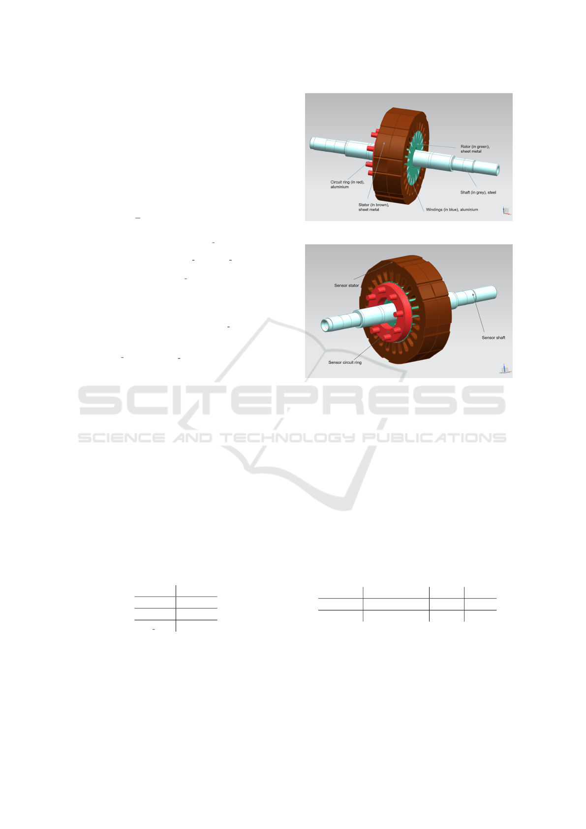
5 APPLICATION: HEATING OF A
MOTOR
The proposed method is applied to the thermal model
of a motor. Fig. 1 shows the motor components and
materials, Fig. 2 the sensor positions. The thermal
conductivity is constant in rotor and stator regions and
temperature-dependent in windings, circuit rings and
shaft, see Fig. 3. For construction of a higher order
approximation in (21), conductance matrices A
min
=
A(T
min
) and A
max
= A(T
max
) are extracted from NX
for T
min
= 20
◦
C and T
max
= 300
◦
C.
~
ξ in (21) is defined
by (19) in windings and circuit rings regions, and by
(18) otherwise. The problem dimensions are shown
in Table 1.
Table 1: Dimensions of full and reduced problem.
n 186527
n
r
60
n
deim
60
n
co deim
332
The loads are applied to the windings. Two test
cases are considered:
• Constant load
• Time-dependent load
In each test case, the initial condition is T (0) = 22
◦
C.
Figure 1: Components of the motor.
Figure 2: Sensor positions.
5.1 Constant Load
In the first test case, a constant load of u = 2e7 W /m
3
is applied to the windings. Fig. 4 shows a compari-
son between NX and the reduced linear model, with
a constant conductance matrix extracted for T = 20
◦
.
Figs. 5 and 6 show results for the full and the re-
duced nonlinear model, respectively. With both mod-
els, higher accuracies are achieved compared to the
reduced linear model, whereby there are only minor
differences between the full and the reduced nonlin-
ear model. The absolute and relative errors are listed
in Table 2.
Table 2: Maximum absolute and relative errors between the
listed models.
Model 1 Model 2 ε
abs
ε
rel
NX MOR(nonlin) 0.9
◦
C 0.8%
NX MOR(lin) 5.6
◦
C 2.9%
5.2 Time-dependent Load
In the second test case, a time-dependent load is ap-
plied (Fig. 7). Again the full and the reduced nonlin-
ear models achieve higher accuracies than the reduced
linear model, see Figs. 8-10 and Table 3.
SIMULTECH 2021 - 11th International Conference on Simulation and Modeling Methodologies, Technologies and Applications
18

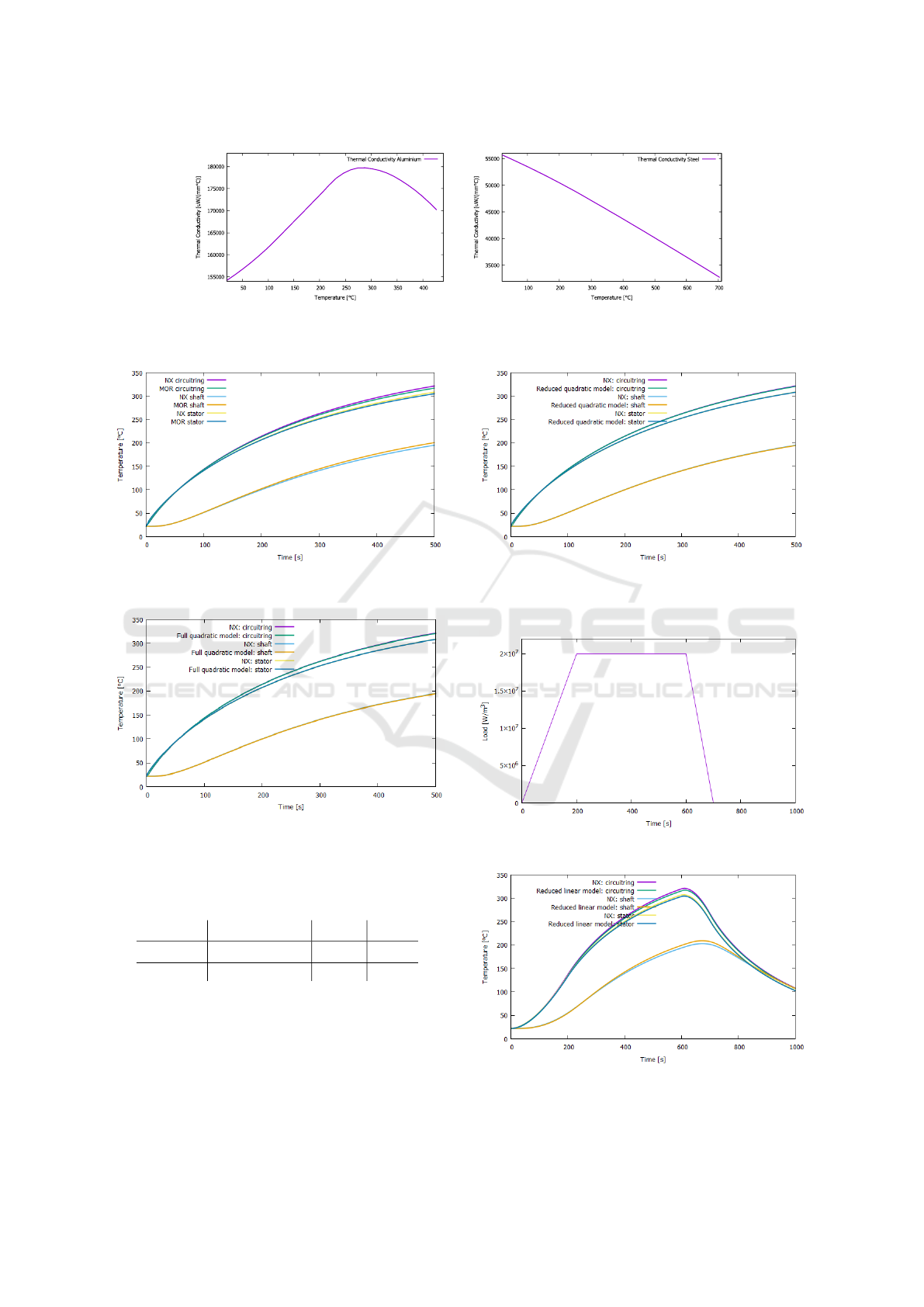
(a) Aluminium (b) Steel
Figure 3: Thermal conductivities of the materials under consideration.
Figure 4: Comparison between NX and reduced linear
model, conductance matrix extracted for T=20
◦
C.
Figure 5: Comparison between NX and full nonlinear
model, conductance matrices extracted for T=20
◦
C and
T=300
◦
C.
Table 3: Maximum absolute and relative errors between the
listed models.
Model 1 Model 2 ε
abs
ε
rel
NX MOR(nonlin) 1.6
◦
C 2.8%
NX MOR(lin) 6.1
◦
C 3.0%
Figure 6: Comparison between NX and reduced nonlin-
ear model, conductance matrices extracted for T=20
◦
C and
T=300
◦
C.
Figure 7: Time-dependent load case.
Figure 8: Comparison between NX and reduced linear
model, conductance matrix extracted for T=20
◦
C.
Reduced Order Modeling for Thermal Problems with Temperature-dependent Conductivities using Matrix Interpolation
19

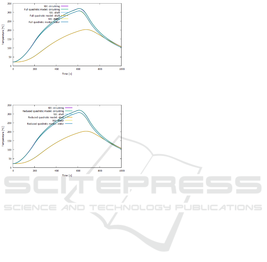
Figure 9: Comparison between NX and full nonlinear
model, conductance matrices extracted for T=20
◦
C and
T=300
◦
C.
Figure 10: Comparison between NX and reduced nonlin-
ear model, conductance matrices extracted for T=20
◦
C and
T=300
◦
C.
6 CONCLUSIONS
In this paper, model order reduction of thermal prob-
lems with temperature-dependent conductivities has
been considered, with the constraint that a com-
mercial solver is used for the full problem where
only matrices for given temperature fields can be ex-
tracted. It has been proposed to approximate the con-
ductance matrix by multi-linear matrix interpolation
which only slightly complicates the solution work-
flow. In the selected examples, the reduced model of
this approximation achieves higher accuracies com-
pared to a model based on a constant approxima-
tion of the conductance matrix. Further improve-
ments maybe achieved by algorithms of deep learn-
ing (L
¨
ohner et al., 2021) which will be the subject of
future investigations.
REFERENCES
Ahmad, M. I., Benner, P., and Jaimoukha, I. (2016).
Krylov subspace methods for model reduction of
quadratic-bilinear systems. IET Control Theory Appl.,
10(16):2010–2018.
Anderl, R. and Binde, P. (2018). Simulations with NX /
Simcenter 3D: Kinematics, FEA, CFD, EM and Data
Management. Carl Hanser Verlag GmbH & Company
KG.
Benner, P., Grivet-Talocia, S., Quarteroni, A., Rozza, G.,
Schilders, W. H. A., and Silveira, L. M. (2021).
Model Order Reduction. Volume 3: Applications. De
Gruyter, Berlin, Boston.
Cao, X., Maubach, J., Weiland, S., and Schilders, W.
(2018). A novel krylov method for model order re-
duction of quadratic bilinear systems. In 2018 IEEE
Conference on Decision and Control (CDC), Miami
Beach, FL, USA.
Chaturantabut, S. and Sorensen, D. C. (2010). Nonlinear
model reduction via discrete empiricial interpolation.
SIAM J. Sci. Comput., Vol. 32(No. 5):2737–2764.
Fritzen, F., Haasdonk, B., Ryckelynck, D., and Sch
¨
ops,
S. (2018). An algorithmic comparison of the hyper-
reduction and the discrete empirical interpolation
method for a nonlinear thermal problem. Mathe-
matical and computational applications, MDPI, Vol.
23(No. 11):pp. 8.
L. Landau, E. L. (1975). The classical Theory of Fields,
volume 2 of Course of Theoretical Physics. Elsevier,
4 edition.
L
¨
ohner, R., Antil, H., Tamaddon-Jahromi, H., Chaksu,
N. K., and Nithiarasu, P. (2021). Deep learning or
interpolation for inverse modelling of heat and fluid
flow problems? Journal of Numerical Methods for
Heat & Fluid Flow.
S. R. de Groot, P. M. (1969). Non-Equilibrium Thermody-
namics. North-Holland Publishing.
SIMULTECH 2021 - 11th International Conference on Simulation and Modeling Methodologies, Technologies and Applications
20