Tailored Military Recruitment through Machine Learning Algorithms

Robert Bryce, Ryuichi Ueno, Christopher Mcdonald and Dragos Calitoiu

Director General Military Personnel Research and Analysis, Department of National Defence,

101 Colonel By Drive, Ottawa, Canada

Keywords:

Machine Learning, Ensemble Learning, Workforce Analytics, Recruitment.

Abstract:

Identifying postal codes with the highest recruiting potential corresponding to the desired proﬁle for a military

occupation can be achieved by using the demographics of the population living in that postal code and the lo-

cation of both the successful and unsuccessful applicants. Selecting N individuals with the highest probability

to be enrolled from a population living in untapped postal codes can be done by ranking the postal codes using

a machine learning predictive model. Three such models are presented in this paper: a logistic regression,

a multi-layer perceptron and a deep neural network. The key contribution of this paper is an algorithm that

combines these models, beneﬁting from the performance of each of them, producing a desired selection of

postal codes. This selection can be converted into N prospects living in these areas. A dataset consisting of

the applications to the Canadian Armed Forces (CAF) is used to illustrate the methodology proposed.

1 INTRODUCTION

Military recruitment refers to the overall process of

attracting and selecting suitable candidates for mili-

tary occupations. At any given time, a broad range

of efforts are deployed in order to continuously im-

prove this process by making it more efﬁcient and

more effective, or, in other words, to ensure the best

use of the available resources to select the best can-

didates for the job. Many of these recruiting efforts,

such as advertising, or career fairs, are addressed to

the general population. Recently, a new line of re-

cruiting efforts became of interest, that of identifying

sub-groups within the general population that have

higher odds than other sub-groups to contain success-

ful candidates for a particular set of jobs, and then

tailor recruiting efforts to these sub-groups. This pa-

per presents a mathematical translation of the process

of identifying the most promising sub-groups, i.e.,

those with the highest potential for prospects that cor-

respond to the desired proﬁle for the occupation(s)

of interest. To be more speciﬁc, the aim is not to

identify individuals per se, but the geographical areas

where they live, at the postal code level of granular-

ity. This will allow, for example, for tailored mail-

ing campaigns to the households in a select set of

postal codes. The selection of this level of granular-

ity was pragmatic, based on the fact that this informa-

https://orcid.org/0000-0003-0173-9846

tion is known for all applicants (whether successful or

not), and that a multitude of external data sources ex-

ist, which provide rich information about neighbour-

hoods, also at the postal code level. The approach

presented here is based on using the postal code as a

primary key (in database terminology) to connect an

applicant with the neighbourhood to which he/she be-

longs which makes possible to augment the applicant

data with the demographic attributes of that neigh-

bourhood. With this augmentation realized, it is pos-

sible to identify the separation between the proﬁle of

the successful applicants (enrollees) and that of non-

successful applicants, using only demographics of the

population living in the postal code. This separation

(a mathematical relationship) can be used to derive

the probability to be enrolled for individuals living

in previously ‘untapped’ postal codes (i.e., no previ-

ous applicants from that postal code), thus uncover-

ing new promising areas where tailored recruited ef-

forts could be applied successfully. The population

in each postal code is known; therefore the number

of individuals can be determined. Identiﬁcation of

N individuals with the highest probability to be en-

rolled, from a population living in untapped postal

codes, can be done by ranking the population using

a machine learning predictive model derived from the

separation described above. Three such models are

presented in this paper, along with an algorithm that

combines them, beneﬁting from the strength of each

Bryce, R., Ueno, R., Mcdonald, C. and Calitoiu, D.

Tailored Military Recruitment through Machine Learning Algorithms.

DOI: 10.5220/0010506500870092

In Proceedings of the 2nd International Conference on Deep Learning Theory and Applications (DeLTA 2021), pages 87-92

ISBN: 978-989-758-526-5

of the individual models, which is considered the key

contribution of this paper.

A brief presentation of the paper follows. We de-

scribe developing three Machine Learning (ML) mod-

els to predict the probability of applicant’s success by

postal codes (Section 2.1). We propose a dynamic

method for combining models in a manner that satis-

ﬁes the requirement N and considers the performance

of each model (Section 2.2).We use a dataset con-

sisting of applications to the Canadian Armed Forces

(CAF) to illustrate the methodology we describe, al-

lowing for a concrete discussion of implementation

issues (Section 3).

2 MACHINE LEARNING

MODELS FOR TAILORED

RECRUITMENT

A machine learning algorithm is an algorithm able

to learn from data. The concept of learning is used

here in the context of improving the algorithm perfor-

mance, for a given task, by using experience (more

data). The task explored in this research is the clas-

siﬁcation in two categories; the learning algorithm is

asked to produce a function f : R

→ {0, 1}. In order

to solve this task, we implemented three architectures:

a logistic regression, a multi-layer perceptron, and a

deep neural network.

The data sets consist of demographics data at the

postal code level, namely of 760 attributes (Environ-

ics Analytics, 2018), as well as a labeled data set of

59,084 postal codes associated with applications to

the CAF in the 2015-18 timeframe. The label is ‘1’

for a successful applicant (enrolled) and ‘0’ for an

unsuccessful applicant. Applicants with no ﬁnal deci-

sion were removed from the data set. The labeled set

was split into development and validation sets, as will

be discussed below.

2.1 Machine Learning Models

Model 1: A logistic regression model (model LR)

was trained as a baseline model. A 14 dimensional

subset of the 760 attributes was chosen by stepwise

selection. Speciﬁcally, for stepwise selection a sig-

niﬁcance level of 0.1 was required to allow a variable

into the model and a signiﬁcance level of 0.01 for a

variable to stay in the model. Collinearity was tested

for, with the acceptable variance inﬂation factor set to

< 2.5 and the acceptable condition index to < 10. The

Hosmer and Lemeshow goodness-of-ﬁt test for the ﬁ-

nal selected model was used. The speciﬁc parame-

ter values used for stepwise selection were based on

standard guidance and diagnostics, for example see

(Chen et al., 2003).

Table 1: Model performance on the validation set. The

percentage of observation and the mean probability are re-

ported for each decile.

Decile LR MLP DNN

Obs. p mean Obs. p mean Obs. p mean

1 15.8 60.0 16.4 64.9 16.1 58.9

2 12.3 44.4 13.2 45.9 13.0 48.7

3 11.2 42.3 11.4 43.1 12.4 46.4

4 10.8 40.8 10.8 40.9 11.2 44.6

5 10.2 39.6 10.2 39.1 10.0 42.8

6 9.4 38.4 8.8 36.7 9.7 40.7

7 9.0 37.0 8.8 34.1 8.4 38.3

8 8.0 35.3 8.1 30.9 7.7 35.0

9 6.9 32.8 6.6 27.5 6.4 30.6

10 6.4 24.5 5.6 22.7 5.2 24.4

Model 2: A classic feed forward multi-layer

perceptron (model MLP) with one hidden layer of

ﬁve nodes and sigmoidal weights was trained via

back-propagation (Rumelhart et al., 1986). The

Adam optimizer was used, with the recommended

default parameters (Kingma and Ba, 2015). L2

regularization was used to penalize large weight

values, with regularization terms of 0.0001. The

MLP was trained on the same 14 dimension subset

of attributes as the LR model, as accuracy was poor

when trained on the full 760 attributes.

Model 3: A Deep Neural Network (model DNN)

classiﬁer, with three hidden layers of 30 nodes each

and rectiﬁed linear unit weights, was also trained

with back-propagation. Again, the Adam optimizer

was used, with the recommended default parameters

(Kingma and Ba, 2015). L2 regularization was used

to penalize large weight values, with regularization

terms of 0.01. The DNN was trained on the full 760

dimensional attributes.

For the LR model the labeled data set was split

into two equal subsets, for development and valida-

tion. In contrast, for the neural networks a 80%-20%

split was used, due to more parameters existing in

these architectures (81 parameters for the MLP and

24,721 for the DNN, versus 15 for the LR model).

The entire validation dataset is scored and a prob-

ability is computed from the score, using the stan-

dard transformation p =

score

1+e

score

, such that each postal

code receives a score and a corresponding probabil-

ity. Next, the validation dataset is sorted in descend-

ing order of the probabilities. We build deciles, the

ﬁrst having the highest probability to enroll and the

last having the lowest probability. We report for each

decile the following numbers: the fraction of enroll-

DeLTA 2021 - 2nd International Conference on Deep Learning Theory and Applications

ments realized on that decile (% Obs.), and the mean

of probabilities predicted by the model (Mean Prob.).

Table 1 contains these values. The lift is deﬁned as

the ratio of enrollments realized in a given segment

(decile here) to the average expected under a uniform

random distribution; for example, the lift for the LR

model on the ﬁrst decile is

15.8%

10.0%

= 1.58. A model

is powerful if it can group in the ﬁrst decile a high

percentage of enrollments. Note that the top deciles

exhibit enhanced lift for all three models.

Observe that the DNN has limited data per weight,

45,818 observations for 24,721 weights, placing train-

ing well outside the classic ‘10x data to weights’ rule

of thumb regime (Baum and Haussler, 1989).

2.2 Ensemble of Models

The underlying motivation of this work is to ﬁnd a

means of combining ML models, to beneﬁt from dif-

ferent strengths of each model. We ﬁrst provide the

algorithm for concreteness and then discuss the moti-

vation behind this approach. The algorithm proposed

is general, namely it can combine any number of

models. The motivation of the algorithm is presented

below. There are two main constraints for the design:

the target audience N (and a corresponding estima-

tion of B postal codes) and the error within any given

model. Predictions for any speciﬁc postal code may

be in error and predicted orderings may have local

‘mixing’ and mis-ordering. By asking for an agree-

ment set between several models up to a given num-

ber B of postal codes (A1), we place the focus near

the ‘top’ postal codes where we are most interested in

good performance. This approach, majority voting,

is a common ensemble averaging scheme (Wolpert,

1992), but we note that it does not account for the

fact that each model has different performance. By

introducing the predictive strength of the models, the

algorithm uses the lift in the segment under consider-

ation (observed success in segment/overall observed

success) in order to weight rankings (A2). We sub-

tract the normalized lift from one in order to account

for the fact that high rankings have a low index value.

Note that by focusing on lift and rank order, we do not

require a precise calibration of the predicted proba-

bilities. The weighted ranks (A3) will not necessarily

be integers; this is not substantial as sorting on non-

integers will lead to interpretable ranking.

Inputs:

• The number of postal codes to target, B, estimated from

the target audience N.

• The lift proﬁles for each model.

• Predictions for each model (postal code, p

, p

, ... ,

), where p

is the vector of the i

ML model pre-

diction of applicants’ success, and M is the number of

models. (In our setting M = 3).

Output:

• Top B ranked postal codes.

Algorithm to Determine the Top B Postal Codes:

• A0: Rank and sort the postal codes for each model, us-

ing the p

vector.

• A1: Find the intersection which contains the top B

postal codes, as ranked by each p

. This ‘agreement

set’ consists of the top S postal codes, with S ≥ B.

• A2: Determine the lift for each model `

for the

deciles containing the S postal codes. Deﬁne normal-

ized weights w

M−1

(1 −

∑

), where the sum is

over the M models in the ensemble.

• A3: Find the ﬁnal weighed ranking r

for the postal

codes in the agreement set, r

∑

· w

where i in-

dexes the postal codes and k the models.

• A4: Sort and output the reranked top B postal codes.

3 RESULTS

As discussed in previous section, we trained three ML

models (a LR, a MLP, and a DNN model). In the

example here, we consider B = 2000 postal codes to

target; the speciﬁc value in practice will be dictated by

N. We apply the algorithm to 694,621 unlabelled and

‘untapped’ (with respect to our labeled data subset)

postal codes. The number of untapped postal codes is

derived by subtracting the number of postal codes in

our labeled data from the total number of postal codes

in Canada.

For the selection of B postal codes derived with

the algorithm presented above, the number N

of in-

dividuals can be computed. Environics demographic

data contains the population per age group for each

postal code. If N

is different than the initial target

audience N, an adjustment on B can be applied, in-

creasing or decreasing it.

The lift which characterizes model performance

is considered in deciles here, for stability reasons,

though percentiles or other more granular breakdowns

are potentially useful, given sufﬁcient data. Use of

deciles is standard practice in industry as the ‘cream

of the crop’ is the focus. Figure 1 plots the cumula-

tive lift percentage by decile for each model. It was

observed that the DNN performs better than the other

two models over the majority of deciles, as can be

more clearly seen in the inset which shows the resid-

ual between the observed lift and the uniform random

model with no lift. Further, the relative performance

depends on which decile cutoff is considered. This

Tailored Military Recruitment through Machine Learning Algorithms

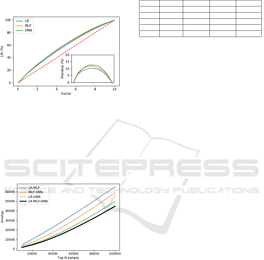
demonstrates the utility of adaptively selecting the lift

to match the region we are interested in. For example,

if the overlap is identiﬁed in the ﬁrst two deciles the

lift corresponding to these two deciles must be used.

Figure 1: Cumulative lift by decile for each model. The dot-

ted red line is the null case random model; the inset shows

the residual between the models and the null case.

Note that logistic regression is a linear model

while neural networks can account for nonlinear sepa-

ration boundaries. With that in mind, the MLP model,

with its ﬁve nodes, has more similar behaviour to the

LR model than the DNN when overlap is considered

(see Figure 2) yet still appears to display more ca-

pacity to separate than the LR (linear) model (see

Figure 1, where performance approaches that of the

DNN).

Figure 2: Agreement set size between models.

For illustration of the algorithm, Table 2 shows

ﬁve postal codes randomly selected from the agree-

ment set, their ranks in the three models, and their re-

ordered ranking; for conﬁdentiality, the postal codes

are not presented explicitly, but denoted as (pc1, pc2,

. . . ).

We should emphasize that the approach taken here

is not intended to be static, but rather a dynamic learn-

ing approach which improves over time. Based on

future campaigns using this approach we will update

predictions. In particular, as we obtain more data the

underlying models and their lifts will be improved.

Table 2: Example postal code rankings and reranking for

ﬁve untapped postal codes.

P. Code LR Rank MLP Rank DNN Rank Ens. Rank

pc1 8 15 25 5

pc2 99 97 242 73

pc3 2813 623 875 470

pc4 1338 421 3773 543

pc5 736 3250 10665 1337

4 DISCUSSION

4.1 Weights

We focus on the ‘best’ predicted B postal codes and

this makes the lift in the top percentiles a natural

means of estimating a model’s performance. We also

want to eliminate any postal code that is not near the

top across models; to do this, we use the intersection,

which may be too conservative, and in which case ma-

jority voting may become a viable alternative. Cali-

bration of probabilities (e.g., ensuring absolute accu-

racy of numbers) is difﬁcult and, in general, there has

been little work done in this area. For this reason,

we do not use the absolute probabilities in determin-

ing performance or reranking, but rather the relative

rankings. The resulting algorithm emphasizes perfor-

mance precisely where we are interested in it (as dic-

tated by the target audience N and the corresponding

number of postal codes B).

The weights introduced here linearly reward rela-

tive performance of the models; these are adaptively

adjusted by using the performance in the segmenta-

tion under consideration (e.g., the top S postal code

regime). To be more speciﬁc, if S covers p deciles, the

weights are derived from lifts generated for p deciles.

In contrast, equal weighing is widely used in ensem-

ble averaging (Wolpert, 1992), which does not ac-

count for different performance of models. We opted

for using reward/penalty of relative performance, for

adaptive reasons (discounting models which become

poor under selection criteria drift; see the next para-

graph for more discussion).

It should be noted that by using normalized lift,

we impose a non-negative and sum one condition on

the weights with values related to relative (predictive)

strength, by construction. Alternative weighting (re-

laxing non-negative or sum one conditions) could po-

tentially be argued as a viable alternative. Early work

on linear stacking (averaging models via weights)

found that if one forces non-negative weights and op-

timizes on training data then, empirically, the sum

one condition approximately holds in practice; more-

over, if non-negativity was not enforced performance

was poor (Breiman, 1996). That work further con-

DeLTA 2021 - 2nd International Conference on Deep Learning Theory and Applications

vincingly argued that the sum one constraint will be

approximately enforced as long as some low predic-

tion error models exist in the ensemble. Note that in

(Dawes, 1979) it was suggested that non-negativity

constraints are required: assuming a model’s perfor-

mance is not anti-correlated with the true behaviour

the weight should be non-negative in a linear ﬁt. In

general, by imposing a sum one condition on the

weights we ensure our ﬁnal model will also be ap-

proximately equal to the expectation of the underly-

ing distribution. The non-negative constraint is self-

evident as long as models are not in severe error (anti-

correlated), and such models are excluded by con-

struction. Selection based on optimality (e.g., relative

predictive strength, as measured by lift here) is likely

to have a lesser affect, but can be argued on adap-

tive grounds: such weightings will adaptively adjust

to model performance, so, for example, if the selec-

tion criteria drift over time, selection of weights via

optimization will downweight models that become

ineffective and reward models that show improved

performance and will therefore reduce model mis-

speciﬁcation risk. Moreover, as we use lift, for var-

ious values of N, we adaptively reweight to take rela-

tive performance into account.

4.2 Implementation Details

The algorithm was implemented in Python 3.6. We

found no implementation or computational issues.

The LR model was implemented in SAS 9.4 and

again no computational difﬁculties were encountered.

In contrast, implementing the neural network mod-

els was somewhat problematic on the Windows lap-

top used (dual core 2.9 GHz i7, 8 GB Random Ac-

cess Memory (RAM), Windows 7 Enterprise). Python

was used with the Scikit-Learn 0.19.2 package (Pe-

dregosa et al., 2011) for training the MLP and the

1.12.0 TensorFlow package (Abadi et al., 2015) for

training the DNN. For the DNN model, due to the

large dimension of the training data (760 attributes)

and number of nodes, our limited computational re-

sources led to slow training and system stability was

compromised to the extent that restarts were neces-

sary. ML libraries often target Graphical Processor

Units (GPUs) to allow more efﬁcient computations,

and the laptop used lacked both GPUs and adequate

RAM. Despite the computational loads stressing our

machine, training was successful although moving

to larger dimensions (more attributes) or training set

sizes would be difﬁcult.

4.3 Potential Extensions

We brieﬂy raise a few items of interest for extending

the approach taken:

• We do not perform dimension reduction or any

other feature engineering, other than the stepwise

reduction used for the LR and MLP; such consid-

erations can improve the performance of the un-

derlying models in the ensemble and additional

work in this area could be beneﬁcial.

• There are many variations one can make to our

algorithm. For example, instead of ﬁnding the in-

tersection in step A1, majority voting can be used

to ﬁnd the agreement set. The model accuracy can

be used to determine weights in step A2, etc. The

crucial aspects are a winnowing of data to keep

the ‘top’ rated postal codes with a voting between

models to ensure enough high value data is con-

sidered, and the integrated use of a budget and

error consideration when selecting and using this

subset of data to determine weights. In addition,

the algorithm is generic, in that any number of

models can be used. If M, the number of mod-

els, is large then the agreement set is expected to

be too conservative, and the use of majority vot-

ing would become increasingly attractive. This is

particularly true if we want to use an ensemble of

weak learners.

• In Canada, postal codes are categorized into urban

and rural regions. Splitting the data into urban and

rural regions may be beneﬁcial. If the number of

postal codes in rural regions is small, eliminating

them from the original data set may improve per-

formance of the model. If the number of postal

codes in rural regions is big enough, developing

separate urban and rural models can be another

option.

• A different direction for research is to explore the

saturation and the frequency of the mailings in a

ﬁxed period of time. The ﬁnal selection N can be

adjusted considering these aspects.

• It should be noted that the approach explored

here is related to stacked generalization (Wolpert,

1992), which is the generic idea of using model

outputs (predicted probability of success here) as

features to construct a meta-model. Here we are

selecting a linear model corresponding to averag-

ing, with weights found by an algorithm that ac-

counts for model error and a ﬁnite N, but other

meta-models can be used (for example logistic re-

gression is a reasonable approach, as probabili-

ties will be the output, and neural networks or any

other suitable machine learning algorithm can be

considered).

Tailored Military Recruitment through Machine Learning Algorithms

5 CONCLUSION

The main contribution of this paper is an algorithm

that combines three predictive models (a logistic re-

gression, a multi-layer perceptron and a deep neural

network) by assigning weights to the ranks produced

by each model. The assignation of the weights is done

considering the lift of each individual model. The al-

gorithm is not intended to be static, but rather a dy-

namic learning approach which improves over time:

the lift will be updated after each additional recruit-

ing campaign.

We tested the algorithm on B = 2000 postal codes

and we identiﬁed an overlap of 21,554 postal codes

in the ﬁrst decile. The models architectures are con-

siderably different and in this context the overlap is

impressive. Using the lift in the ﬁrst decile of our

predictive models we produced a list of ranked postal

codes. This algorithm for combining the models will

be validated with the data collected in future recruit-

ment campaigns. The same data will be used for ad-

justing the lift for each individual model in the ensem-

ble.

REFERENCES

Abadi, M., Agarwal, A., Barham, P., Brevdo, E., Chen,

Z., Citro, C., Corrado, G. S., Davis, A., Dean, J.,

Devin, M., Ghemawat, S., Goodfellow, I., Harp, A.,

Irving, G., Isard, M., Jia, Y., Jozefowicz, R., Kaiser,

L., Kudlur, M., Levenberg, J., Mane, D., Monga,

R., Moore, S., Murray, D., Olah, C., Schuster, M.,

Shlens, J., Steiner, B., Sutskever, I., Talwar, K.,

Tucker, P., Vanhoucke, V., Vasudevan, V., Viegas, F.,

Vinyals, O., Warden, P., Wattenberg, M., Wicke, M.,

Yu, Y., and Zheng, X. (2015). Tensorﬂow: Large-

scale machine learning on heterogeneous systems.

https://www.tensorﬂow.org. Accessed Feb. 20, 2019.

Baum, E. and Haussler, D. (1989). What size net gives valid

generalization? Neural Computation, 1(1):151–160.

Breiman, L. (1996). Stacked regressions. Machine Learn-

ing, 24:49–64.

Chen, X., Ender, P., Mitchell, M., and Wells, C. (2003).

Regression with SAS. https://stats.idre.ucla.edu/sas/

webbooks/reg/. Accessed Feb. 20, 2019.

Dawes, R. M. (1979). The robust beauty of improper linear

models in decision making. American Psychologist,

34(7):571–582.

Environics Analytics (2018). Demstats database.

https://www. environicsanalytics.com. Accessed

Feb. 20, 2019.

Kingma, D. and Ba, J. (2015). Adam: A method

for stochastic optimizaton. https://arxiv.org/

pdf/1412.6980.pdf. Accessed Feb. 20, 2019.

Pedregosa, F., Varoquaux, G., Gramfort, A., Michel, V.,

Thirion, B., Grisel, O., Blondel, M., Prettenhofer, P.,

Weiss, R., Dubour, V., Vanderplas, J., Passos, A.,

Cournapeau, D., Brucher, M., Perrot, M., and Duch-

esnay, E. (2011). Scikit-learn: Machine learning

in Python. Journal of Machine Learning Research,

12:2825–2830.

Rumelhart, D. E., Hinton, G., and Williams, R. (1986).

Learning representations by back-propagating errors.

Nature, 323(9):533–536.

Wolpert, D. H. (1992). Stacked generalization. Neural Net-

works, 5:241–259.

DeLTA 2021 - 2nd International Conference on Deep Learning Theory and Applications