Comprehensive Empirical Analysis of Stop Criteria in Computerized
Adaptive Testing
Patricia Gilavert
a
and Valdinei Freire
b
School of Arts, Sciences and Humanities, University of S
˜
ao Paulo, S
˜
ao Paulo, Brazil
Keywords:
Computerized Adaptive Testing, Stop Criteria, Combine Stop Criteria, Threshold to Stop.
Abstract:
Computerized Adaptive Testing is an assessment approach that selects questions one after another while con-
ditioning each selection on the previous questions and answers. CAT is evaluated mainly for its precision,
the correctness of estimation of the examinee trait, and efficiency, the test length. The precision-efficiency
trade-off depends mostly on two CAT components: an item selection criterion and a stop criterion. While
much research is dedicated to the first, stop criteria lack relevant research. We contribute with a comprehen-
sive evaluation of stop criteria. First, we test a variety of seven stop-criteria for different setups of item banks
and estimation mechanism. Second, we contribute with a precision-efficiency trade-off method to evaluate
stop criteria. Finally, we contribute with an experiment considering simulations over a myriad of synthetic
item banks. We conclude in favor of the Fixed-Length criterion, as long it can be tuned to the item bank at
hand; the Fixed-Length criterion shows a competitive precision-efficiency trade-off curve in every scenario
while presenting zero variance in test length. We also highlight that estimation mechanism and item-bank
distribution have a influence over the performance of stop criteria.
1 INTRODUCTION
Computerized Adaptive Testing (CAT) is an approach
to assessment that tailors the administration of test
items to the trait level of the examinee. Instead of
applying the same question to every examinee, as in
a traditional paper and pencil test, CATs apply ques-
tions one after another and each question selection is
conditioned on the previous questions and answers
(Segall, 2005). The number of applied questions to
each examinee can also be variable to reach a better
trade-off between precision, a correct trait estimation,
and efficiency, a small number of questions. CATs
reduce the burden of examinees in two ways; first, ex-
aminees do not need to complete a lengthy test; sec-
ond, examinees answer questions tailored to their trait
level avoiding too difficult or too easy questions (Spe-
nassato et al., 2015).
Because examinees do not solve the same set of
questions; an appropriate estimation of the latent trait
level of the examinee must be considered. In the
case of dichotomic questions, the item response the-
ory (IRT) can be used to find the probability of an
examinee to score one item as a function of his/her
a
https://orcid.org/0000-0001-8833-9209
b
https://orcid.org/0000-0003-0330-3931
trait and therefore provide a coherent estimator. CAT
in combination with IRT makes it possible to cal-
culate comparable proficiencies between examinees
who responded to different sets of items and at differ-
ent times (Hambleton and Swaminathan, 2013; Kre-
itzberg et al., 1978). This probability is influenced by
item parameters, as difficulty and discrimination.
In every CAT we identify at least six components
(Wainer et al., 2000; Wang et al., 2011): (i) an item
bank, (ii) an entry rule, (iii) a response model, (iv) an
estimation mechanism, (v) an item selection crite-
rion, and (vi) a stop criterion. The item bank deter-
mines questions that are available for the test; usu-
ally, items are selected without replacement. The en-
try rule specifies a priori knowledge from the exami-
nee; in a Bayesian framework, it represents an a pri-
ori distribution over latent traits, and, in a Likelihood
framework, it represents an initial estimation. The re-
sponse model describes the probability of scoring for
each examinee on each question in the item bank; the
response model supports the estimation mechanism to
estimate the latent trait of the current examinee. The
item selection criterion chooses the question to be ap-
plied to the current examinee, while the stop criterion
chooses when to stop the test; usually, both criteria
may be supported by the current estimation, the item
48
Gilavert, P. and Freire, V.
Comprehensive Empirical Analysis of Stop Criteria in Computerized Adaptive Testing.
DOI: 10.5220/0010500200480059
In Proceedings of the 13th International Conference on Computer Supported Education (CSEDU 2021) - Volume 1, pages 48-59
ISBN: 978-989-758-502-9
Copyright
c
 2021 by SCITEPRESS – Science and Technology Publications, Lda. All rights reserved

bank, and the response model.
CAT may be evaluated for its precision and effi-
ciency and both metrics depend on the six compo-
nents of the CAT. Much research on CAT is devoted to
providing and evaluating different selection criteria;
while stop criteria are much less explored. However,
the CAT criterion is the main responsible to choose
the trade-off between precision and efficiency.
We contribute with a comprehensive evaluation of
stop criteria. Because the performance of stop cri-
teria may depend on the other five components of the
CAT; we test a variety of seven stop-criteria while also
varying two of the other components: item banks and
estimation mechanism.
While the response model and the entry rule may
influence the stop criteria performance, both present
natural choices in practice. For the response model,
since we considered dichotomous items, we choose
the IRT ML3 model. For the entry rule, we considered
the standard normal distribution, which is commonly
used to calibrate item banks. Although selection cri-
teria present many options, all of them show the same
behavior: the greater the number of questions, the bet-
ter the precision; stop criteria are all about balancing
the level of precision and the possibility of improve-
ment for the population of examinees. We evaluate
stop criteria fixing the selection criterion with Fisher
Information (FI) criterion; FI criterion is widely used
because it is the cheapest computationally.
We also contribute with a precision-efficiency
trade-off method to evaluate stop criteria. Most of the
stop criteria consider a metric and a threshold; if the
metric is below the threshold, then the test ends. Usu-
ally, works evaluating stop criteria consider a small
set of thresholds for each stop criterion and measure
efficiency and precision for each configuration; be-
cause nor efficiency neither precision is fixed, it turns
up that such configurations are incomparable. Our
method considers configuration to come up with ef-
ficiency levels along all the spectrum of the number
of questions and precision resulting in a precision-
efficiency trade-off curve for each stop criterion. Such
a trade-off curve allows comparing stop criteria along
the relevant spectrum of thresholds.
Another interesting contribution is an experiment
considering simulation over a myriad of synthetic
item banks. First, we consider different setups to gen-
erate item banks; we variate over three probability-
distribution classes for parameter difficulty of items
and over three levels of centrality for each class. Sec-
ond, for each setup, we simulate 500 item banks; sur-
prisingly, works in the literature consider only one
item bank for each setup which can increase bias. Al-
though not being the focus of this paper, we take ad-
vantage of such a myriad of item banks to also evalu-
ate different selection criteria under the Fixed-Length
stop criterion.
The small number in the literature of papers eval-
uating stop criteria by itself justifies our contribu-
tions. The work of (Babcock and Weiss, 2009) is an
inspiration to select different classes of probability-
distribution for item difficulty. They make use of two
classes (uniform and peak) and two lengths of item
banks (100 e 500). However, they simulate only one
instance of each item bank setup. The work of (Mor-
ris et al., 2020) is an inspiration to select different cen-
trality for item difficulty. They experiment with a real
item bank to assess patient-reported outcomes; such
an item bank has a positive centrality over item diffi-
culty.
2 COMPUTERIZED ADAPTIVE
TESTING
CATs are applied in an adaptive way to each exam-
inee by computer. Based on predefined rules of the
algorithm, the items are selected sequentially during
the test after each answer to an item (Spenassato et al.,
2015). A classic CAT can be described by the follow-
ing steps (van der Linden and Glas, 2000):
1. The first item is selected;
2. The latent trait is estimated based on the first item
answer;
3. The next item to be answered is selected. This
item should be the most suitable for the punctual
ability estimation;
4. The latent trait is recalculated based on previous
answers;
5. Repeat steps 3 and 4 until an answer is no longer
necessary according to a pre-established criterion,
called stop criterion.
2.1 Item Response Theory
It is possible to build a CAT based on the item re-
sponse theory (IRT), a mathematical model that de-
scribes the probability of an individual to score an
item as a function of the latent trait level. This prob-
ability is also influenced by the item parameters, as
difficulty, discrimination capacity and random correct
answer. This is the case of the logistic model with
three parameters (Birnbaum, 1968), given by:
Pr(X
i
= 1 | θ) = c
i
+
(1 − c
i
)
1 + exp[−Da
i
(θ − b
j
)]
, (1)
where,
Comprehensive Empirical Analysis of Stop Criteria in Computerized Adaptive Testing
49

• θ is the latent trait of the examinee, in the case of
a test, θ is the examinee’s ability;
• X
i
is a binary variable, 1 indicates that the exam-
inee answers correctly to the item i and 0 other-
wise;
• Pr(X
i
= 1 | θ) is the probability that an individual
with latent trait θ answers correctly the item i;
• a
i
is the discrimination parameter of the item i;
• b
i
is the difficulty parameter of the item i;
• c
i
is the probability of a random correct answer of
the item i; and
• D is a scale factor that equals 1 for the logistic
model, and 1.702 so that the logistic function ap-
proximates the normal ogive function.
Given a examinee θ and a sequence of n answers x
n
=
x
i
1
, x
i
2
, . . . , x
i
n
, the latent trait θ can be estimated by
Bayesian procedure or Maximum Likelihood (ML)
(de Andrade et al., 2000).
We consider here a Bayesian estimator based on
expected a posteriori (EAP), i.e.,
ˆ
θ = E [θ|x
n
] =
Z
θ
f (θ)
∏
n
k=1
Pr(X
i
k
= x
i
k
|θ)
Pr(X
n
= x
n
)
d(θ),
(2)
where f (θ) is the a priori distribution on the latent
trait θ, usually considered the standard normal distri-
bution.
The ML estimator estimates the latent trait by
ˆ
θ =
max
θ
L(θ|x
n
) where the likelihood is given by:
L(θ|x
n
) =
n
∏
k=1
Pr(X
i
k
= x
i
k
|θ). (3)
2.2 Item Selection Criteria
The choice of the item selection method can have an
effect in the efficiency and precision of the examinee
ability estimation. We consider five different item se-
lection criteria. Three of them are based on Fisher In-
formation, while two of them are based on Kullback-
Leibler divergence.
Each criterion defines a score function S
i
(x
n
) for
each item given previous n answers of the examinee,
then, between the items that was not yet applied to the
examinee, the one with the greatest score is is chosen.
At each stage n + 1, when selecting an item, the
item selection criteria may make use of:
ˆ
θ
n
, the latent
trait estimation after n answers; f (θ|x
n
), the a pos-
teriori distribution after n answers; and L(θ|x
n
), the
likelihood after n answers. To simplify notation we
describe shortly P
i
(θ) = Pr(X
i
= 1 | θ).
We also define the Kullback-Leibler divergence
between the score distribution of item i for two ex-
aminees with latent trait θ and
ˆ
θ by
KL
i
(θ||
ˆ
θ) = P
i
(
ˆ
θ)ln
"
P
i
(
ˆ
θ)
P
i
(θ)
#
+ Q
i
(
ˆ
θ)ln
"
Q
i
(
ˆ
θ)
Q
i
(θ)
#
(4)
where Q
i
(θ) = 1 − P
i
(θ).
Fisher Information (FI) (Lord, 1980): this method
selects the next item that maximizes Fisher informa-
tion given the latent trait estimation (Sari and Raborn,
2018), i.e.,
S
i
(x
n
) = I
i
(
ˆ
θ
n
) =
h
d
d
ˆ
θ
n
P
i
(
ˆ
θ
n
)
i
2
P
i
(
ˆ
θ
n
)(1 − P
i
(
ˆ
θ
n
))
(5)
where I
i
(θ) is the information provided by the item i
at the ability level θ.
Kullback–Leibler (KL) (Chang and Ying, 1996):
is based on a log-likelihood ratio test. In the CAT
framework, this method calculates the nonsymmet-
ric distance between two likelihoods at two estimated
trait levels, called KL information gain. KL is the ra-
tio of two likelihood functions instead of a fixed value
as in the FI (Sari and Raborn, 2018). KL criterion de-
fines the following score function:
S
i
(x
n
) =
Z
∞
−∞
KL
i
(θ||
ˆ
θ
n
)L(θ|x
n
)d(θ). (6)
Posterior Kullback–Leibler (KLP) (Chang and
Ying, 1996): the KLP method weights the current KL
information by the a posteriori distribution of θ (Sari
and Raborn, 2018). KLP criterion defines the follow-
ing score function:
S
i
(x
n
) =
Z
∞
−∞
KL
i
(θ||
ˆ
θ
n
) f (θ|x
n
)d(θ). (7)
Maximum Likelihood Weighted Information
(MLWI) (Veerkamp and Berger, 1997): while
FI considers the Fisher information at the current
estimation
ˆ
θ
n
, MLWI weights Fisher information at
different levels by the likelihood function (Sari and
Raborn, 2018), i.e.,
S
i
(x
n
) =
Z
∞
−∞
I
i
(θ)L(θ|x
n
)d(θ). (8)
Maximum Posterior Weighted Information
(MPWI) (van der Linden, 1998): just like MLWI,
MPWI considers a weight Fisher information, but
in this case considering the a posteriori distribution
(Sari and Raborn, 2018), i.e.,
S
i
(x
n
) =
Z
∞
−∞
I
i
(θ) f (θ|x
n
)d(θ). (9)
CSEDU 2021 - 13th International Conference on Computer Supported Education
50

Minimizing the Expected Posterior Variance
(MEPV) (Morris et al., 2020): Bayesian approach
is considered. The CAT presents the item i for which
the expected value of the posterior variance, given we
administer item i, is smallest, i.e.,
S
i
(x
n
) = −E
i
(Var(θ|x
n
)). (10)
2.3 Stop Criteria
While Item Selection Criteria have the objective of
determining a good trade-off between test length and
latent trait estimation, Stop Criteria elect the best
trade-off for a given a test. In this case, a test man-
ager must determine the importance of test length and
estimation quality.
Fixed-Length (FL): is the commonest stop crite-
rion. In this case, every examinee answer a subset of
the N questions, potentially for a different subset of
items. While FL guarantees that every examinees an-
swer the same number of questions, providing some
feeling of fairness, examinees may be evaluated with
different precision, unless the number of answered
question is sufficient large.
The variable-length stop criteria maybe clustered
into two groups: Minimum Precision and Minimum
Information. The first one stops a test only when a
minimum precision on the latent trait estimation was
obtained. The second one stops a test if there is no
more information in the item banks. Stop criteria dif-
ferentiate from each other on how precision and in-
formation is measured.
Standard Error (SE) (Babcock and Weiss, 2009):
considers the precision given by standard deviation of
the latent trait estimator
ˆ
θ
n
. If the real latent trait θ
0
is
known, the standard deviation can be calculate by the
Fisher Information; i.e.,
q
Var(
ˆ
θ
n
) =
1
q
∂
2
logL(θ
0
|x
n
)
∂θ
2
.
Since θ
0
is unknown, it is approximated by
ˆ
θ
n
and
stand error is defined by:
SE(
ˆ
θ
n
) =
1
q
∂
2
logL(
ˆ
θ
n
|x
n
)
∂θ
2
. (11)
Variance a Posteriori (VAP): similar to SE, when
a Bayesian approach is considered, a precision over
estimation can be obtained by the variance of distri-
bution a posteriori f (θ|x
n
). Therefore, we simply de-
fine:
VAP(
ˆ
θ
n
) = Var(θ) =
Z
(θ −
ˆ
θ
n
)
2
f (θ|x
n
)d(θ). (12)
Maximum Information (MI) (Babcock and Weiss,
2009): considers information for each question not
yet submitted to the examinee. The intuition is that if
no question have information, then, the test can stop.
Therefore, we simply define:
MI(
ˆ
θ
n
) = max
i∈Q
n
I
i
(
ˆ
θ
n
), (13)
where I
n
is the set of items not submitted to the ex-
aminee at stage n.
Change Theta (CT) (Stafford et al., 2019): while
MI evaluates questions before submitting them to an
examinee, CT stop criterion evaluates the information
of the last question by the amount of change in esti-
mator
ˆ
θ
n
, i.e.,
CT (
ˆ
θ
n
) = |
ˆ
θ
n
−
ˆ
θ
n−1
|. (14)
Variance of Variance a Posteriori (VVAP): simi-
lar to RCSE, we propose a new stop criterion based
on the variance a posteriori. The objective is to com-
pare the variances a posteriori of calculated θ in the
last administrated items. In case it is not changing,
the test can be stopped because there is no more in-
formation. We consider the variance of the variance a
posteriori of the last 5 estimations and we define:
VVAP(
ˆ
θ
n
) =
4
∑
j=0
(Var(
ˆ
θ
n− j
) − µ
Var,n
)
2
5
, (15)
where
µ
Var,n
=
4
∑
j=0
Var(
ˆ
θ
n− j
)
5
.
3 METHOD
Along with the experimental results, that we show
in the next section, we improve on the method to
evaluate CAT strategies. Different from previous
works, we simulated many item banks among differ-
ent classes of item distributions. Also, instead of con-
sidering a small set of previously defined thresholds
for stop criteria, we choose stop-criteria thresholds af-
ter experiments.
3.1 Item Banks
In this study IRT ML3 model was considered with
the following parameters for each item i: a
i
is the dis-
crimination parameter; b
i
is the difficulty parameter;
and c
i
is the probability of a random correct answer.
We also consider the scale factor D = 1.702.
Comprehensive Empirical Analysis of Stop Criteria in Computerized Adaptive Testing
51

We consider nine classes of item-bank distribu-
tion. In all of them the discrimination parameters
are draw from a log-normal distribution, i.e, a
i
∼
log-normal(0, 0.35); and the probability of a random
correct answer parameters are draw from a beta distri-
bution, i.e., c
i
∼ beta(1, 4). The difficulty parameters
are draw from nine different distribution.
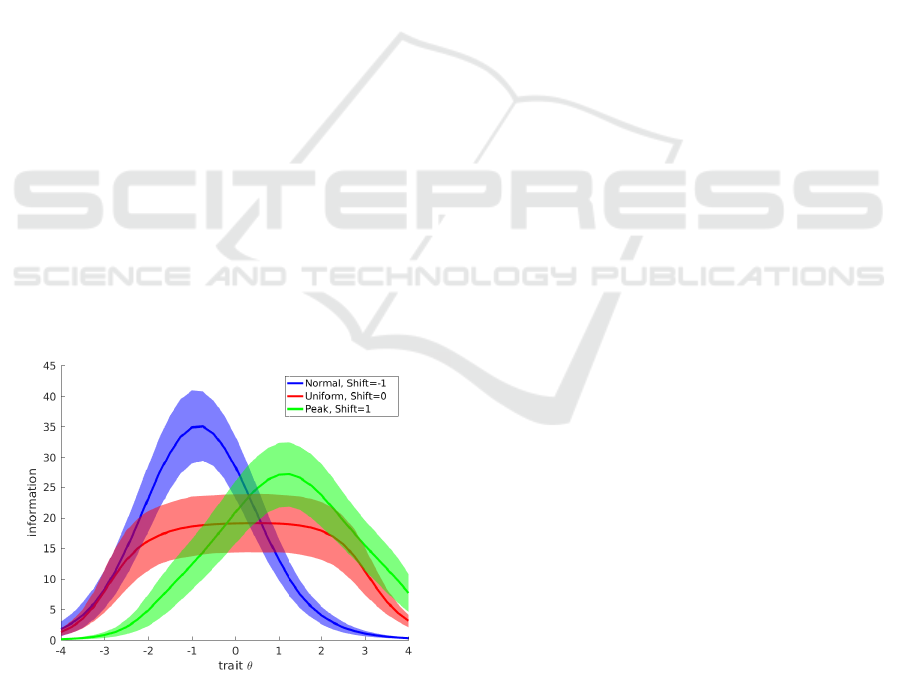
Following Babcock and Weiss (2009) we consider
three classes of distribution for difficulty parameter:
uniform, normal and peak. The uniform class draws
difficulty parameters from a uniform distribution, i.e.,
b
i
∼ uni f orm(−3, 3). The normal class draws diffi-
culty parameters from a standard normal distribution,
i.e., b
i
∼ norm(0, 1). The peak class is a mixed dis-
tribution that with 0.5 probability draws items from
a standard normal distribution and with 0.5 probabil-
ity draws items from a uniform distribution in (-3,3),
as proposed in the Babcock and Weiss (2009); peak
distribution simulates item banks closer to real ones,
where most of the items are around a expected desired
trait, but also present extreme items.
Following Morris et al. (2020), we apply for each
of the three distributions – uniform, norm and peak –
three level of shifts: -1, 0 and 1. Note that, when con-
sidering -1 as the shift level, we increase the chance
of occurring only correct answers for some high-trait
students, since we have a substantial number of easy
questions.
Figure 1 shows the information confidence-
interval for three of this nine distribution with 100
hundred items. Note that, the information for a given
trait θ may vary substantially intra item-bank distri-
bution and inter item-bank distribution.
Figure 1: Mean information of 100-items banks conditioned
on the trait θ and confidence interval with confidence α =
0.1.
3.2 CAT Simulation
We evaluate CAT methods conditioned on one of the
nine item bank class B. For each item bank class we
have done:
1. repeat 500 times:
(a) draw a 100-items bank from B and repeat 50
times
i. draw a trait θ from a standard normal distribu-
tion
ii. simulate a CAT with fixed-length of 50 ques-
tions
iii. log relevant statistics at each question round
We experiment with ML and EAP estimation meth-
ods. For the Bayesian method, the a priori distribu-
tion considered for Pr(θ) is the standard normal dis-
tribution. For the Likelihood method, the initial trait
estimation is 0; in case the student miss (hit) every
question, his/her trait is decreased (increased) by 0.25
until a minimum (maximum) of -2 (2); after at least
one miss and one hit, trait is obtained by the maxi-
mum likelihood.
On each round n of CAT, we log:
• estimated trait
ˆ
θ
n
;
• square error (
ˆ
θ
n
− θ)
2
;
• standard error SE(
ˆ
θ
n
);
• Variance a Posteriori VAP(
ˆ
θ
n
);
• Maximum Information MI(
ˆ
θ
n
);
• Change Theta CT (
ˆ
θ
n
); and
• Variance of Variance a Posteriori VVAP(
ˆ
θ
n
).
3.3 Precision-efficiency Trade-off
Precision and efficiency are the most popular criteria
to evaluate CAT methods. Both depends on the select
criterion and stop criterion; while most select crite-
rion does not present parameters, the stop criterion
requires beforehand a threshold parameter.
Usually, it is easy to obtained a precision-
efficiency trade-off curve when the stop criterion is
the Fixed-Length (for example, Figures 2 and 3). For
variable-length stop criterion, usually, a small set of
threshold parameters are chosen beforehand.
We obtain a precision-efficiency trade-off curve
for each stop criterion by the choosing an appropri-
ate set of threshold levels. Remember that for each
round in every CAT simulation, we log statistics for
each stop-criterion. Then, for each round, we obtain
the median of such statistics and consider such medi-
ans as threshold levels. As we can see in our results,
CSEDU 2021 - 13th International Conference on Computer Supported Education
52

choosing these threshold levels in this way allows to
span our trade-off curve along almost all region of
CAT length.
Together with the stop-criterion, we consider two
additional constraints: (i) exams cannot stop before
the eleventh question; and (ii) exams cannot have
more than 50 questions.
4 RESULTS
4.1 Performance of Selection Criteria
In order to define which item selection criteria to use,
we compare all the criteria defined in section 2.2 and
set the stop criterion to FL, with a maximum of 30
items, and observe the performance of each selection
criterion. We test over all the nine item-bank classes,
here we discuss on results for one of them: Peak with
shift of +1; the results for other item-bank classes can
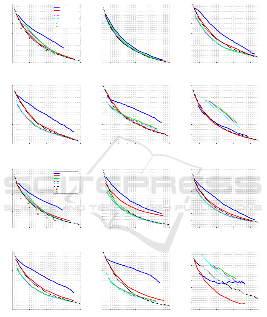
be seen in Appendix (see Figures 12 and 13).
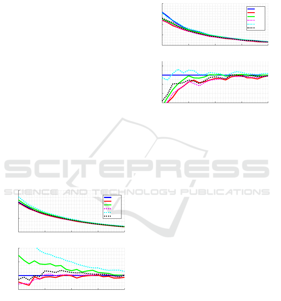
Figures 2 and 3 show the results for each crite-
rion comparing the average length of the CAT and
the average RMSE, using EAP and ML methods,
respectively, to estimate the ability and distribution
peak for difficulty parameter considering +1 as the
shift level. Figures show absolute RMSE and rel-
ative RMSE, when compared to FI method. Using
10 15 20 25 30
CAT Length
0.25
0.3
0.35
0.4
RMSE
FI
MEPV
KL
KLP
MLWI
MPWI
10 15 20 25 30
CAT Length
-5
0
5
10
∆ RMSE
× 10
-3
Figure 2: Comparison of item selection criteria using FL
as a stop criterion and EAP for estimation and distribu-
tion peak for difficulty parameter considering +1 as the shift
level.
the EAP method, it is observed that the FI, KLP and
MEPV criteria are competitive in relation to the oth-
ers. While MLWI and KL show higher mean RMSE
at the beginning of the test; remember that both of
them makes use of likelihood to weight-average over
the trait space.
10 15 20 25 30
CAT Length
0.3
0.35
0.4
0.45
0.5
RMSE
FI
MEPV
KL
KLP
MLWI
MPWI
10 15 20 25 30
CAT Length
-0.03
-0.02
-0.01
0
0.01
∆ RMSE
Figure 3: Comparison of item selection criteria using FL as
a stop criterion and ML for estimation and distribution peak
for difficulty parameter considering +1 as the shift level.
Using the ML method, the KL, KLP and MEPV crite-
ria are more competitive than the others. In this case,
FI has a higher mean RMSE. The MLWI criterion, as
in the previous case, has a higher mean RMSE in most
cases.
All the selection criteria analyzed improve their
accuracy the greater the number of questions. Al-
though MEPV presents a good performance, it is the
most costly because it always chooses the next item
calculating the variance a posteriori considering all
the items administered so far. FI is less costly because
the item choice is based on the current θ estimate.
Therefore, the FI method was chosen as the item
selection criterion to compare the stop criteria as it is
less computationally costly. Although FI method does
not present the best precision, the difference among
methods is small and we belief that it does not inter-
fere in the results of the following sections.
4.2 Performance of Stop Criteria
To compare the performance of the stop criteria, set-
ting FI as the item selection criterion, the mean RMSE
and the mean CAT length were calculated using all
simulated item banks. CAT had to do a minimum of
10 items and a maximum of 50, that is, if the stop
criterion does not finish the test up to 50 items, it is
interrupted. All distributions and shifts in the distri-
butions defined for b have been tested.
Comprehensive Empirical Analysis of Stop Criteria in Computerized Adaptive Testing
53

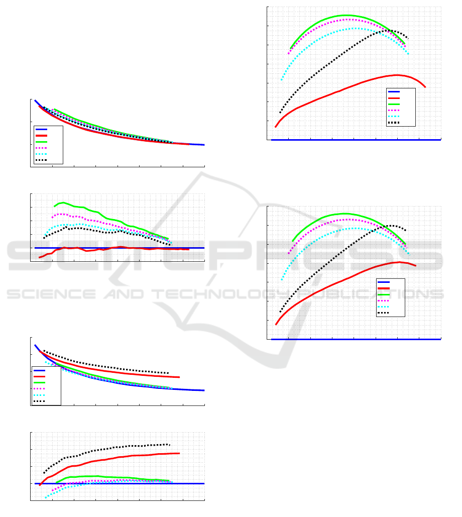
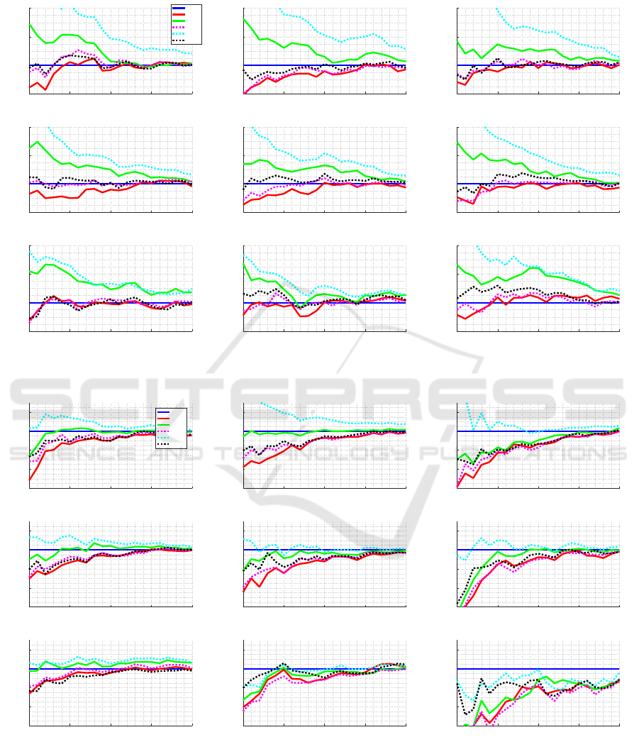
Precision-efficiency Trade-off. We test over all the
nine item-bank classes, here we discuss on results for
one of them: Peak with shift of +1; the results for
other item-bank classes can be seen in Appendix (see
Figures 14 and 15).
Figures 4 and 5 show the results for each stop cri-
terion comparing the length of the CAT and the aver-
age RMSE, using EAP and ML methods, respectively,
to estimate the ability and distribution peak for diffi-
culty parameter considering +1 as the shift level. Fig-
ures show absolute RMSE and relative RMSE, when
compared to FL method.
10 15 20 25 30 35 40 45 50
CAT Length
0.2
0.25
0.3
0.35
RMSE
FL
CT
SE
VAP
VVAP
MI
10 15 20 25 30 35 40 45 50
CAT Length
-5
0
5
10
15
20
∆ RMSE
× 10
-3
Figure 4: Comparison of stop criteria using FI as an item
selection criterion and EAP for estimation and distribution
peak for difficulty parameter considering +1 as the shift
level.
10 15 20 25 30 35 40 45 50
CAT Length
0.25
0.3
0.35
0.4
0.45
RMSE
FL
CT
SE
VAP
VVAP
MI
10 15 20 25 30 35 40 45 50
CAT Length
-0.02
0
0.02
0.04
0.06
∆ RMSE
Figure 5: Comparison of stop criteria using FI as an item
selection criterion and ML for estimation and distribution
peak for difficulty parameter considering +1 as the shift
level.
Standard Deviation of CAT Length. Figures 6 and
7 show the CAT length standard deviation for each
stop criterion using EAP and ML estimation, respec-
tively.
10 15 20 25 30 35 40 45 50
CAT Length
0
2
4
6
8
10
12
14
Std CAT Length
FL
CT
SE
VAP
VVAP
MI
Figure 6: CAT length standard deviation for each stop cri-
terion using EAP estimation and distribution peak for diffi-
culty parameter considering +1 as the shift level.
10 15 20 25 30 35 40 45 50
CAT Length
0
2
4
6
8
10
12
14
Std CAT Length
FL
CT
SE
VAP
VVAP
MI
Figure 7: CAT length standard deviation for each stop crite-
rion using ML estimation and distribution peak for difficulty
parameter considering +1 as the shift level.
As expected, the standard deviation for FL criterion
is 0. The criteria with the least variation are MI and
CT; remember that they both evaluate how much in-
formation rest in item bank, the first one by evalu-
ating fisher information, the later one by evaluating
improvement in the trait estimation. Methods based
on variance estimation presents the highest standard
deviation; in the worst case, SE, a CAT with mean
length of 30, may present a standard deviation of 13
items.
CAT Length vs. Trait. Although FL method
present a competitive precision-efficiency trade-off
and no variance, other stop criterion may be advanta-
CSEDU 2021 - 13th International Conference on Computer Supported Education
54

10 20 30 40 50
Mean CAT Length
-20
-15
-10
-5
0
5
10
15
20
Difference in CAT Length
1st range
FL
CT
SE
VAP
VVAP
MI
10 20 30 40 50
Mean CAT Length
-20
-15
-10
-5
0
5
10
15
20
Difference in CAT Length
2nd range
10 20 30 40 50
Mean CAT Length
-20
-15
-10
-5
0
5
10
15
20
Difference in CAT Length
3rd range
10 20 30 40 50
Mean CAT Length
-20
-15
-10
-5
0
5
10
15
20
Difference in CAT Length
4th range
10 20 30 40 50
Mean CAT Length
-20
-15
-10
-5
0
5
10
15
20
Difference in CAT Length
5th range
Figure 8: Difference in CAT length regarding the mean CAT length by dividing the trait distribution into 5 ranges using EAP
estimation and distribution peak for difficulty parameter considering -1 as the shift level.
10 20 30 40 50
Mean CAT Length
-20
-15
-10
-5
0
5
10
15
20
Difference in CAT Length
1st range
10 20 30 40 50
Mean CAT Length
-20
-15
-10
-5
0
5
10
15
20
Difference in CAT Length
2nd range
FL
CT
SE
VAP
VVAP
MI
10 20 30 40 50
Mean CAT Length
-20
-15
-10
-5
0
5
10
15
20
Difference in CAT Length
3rd range
10 20 30 40 50
Mean CAT Length
-20
-15
-10
-5
0
5
10
15
20
Difference in CAT Length
4th range
10 20 30 40 50
Mean CAT Length
-20
-15
-10
-5
0
5
10
15
20
Difference in CAT Length
5th range
Figure 9: Difference in CAT length regarding the mean CAT length by dividing the trait distribution into 5 ranges using EAP
estimation and distribution peak for difficulty parameter considering -1 as the shift level.
geous if the examiner wants differentiate examinees.
For instance, the examiner may desire that that exam-
inees with the lowest trait spend less time answering
the test.
Figures 8 and 9 show the difference in CAT length
regarding the mean CAT length by dividing the trait
space into 5 ranges with the same amount of traits
after following standard deviation distribution. The
first graph refers to the lowest traits and the last graph
refers to the highest traits.
We consider peak distribution with shift level
equal to -1 (Figure 8) and +1 (Figure 9). In the first
case, there is less information for examinees in the 5th
range, while in the second case, there is less informa-
tion for examinees in the 1st range (see Figure 1).
Stop criteria based in information, such as MI and
CT, make use of less items for examinees with few in-
formation in the item bank; on the other side, stop cri-
teria based on variance, such as SE, VAP, and VVAP,
make use of less items for examinees with large infor-
mation in the item bank. Figures 8 and 9 show such
opposite behaviour.
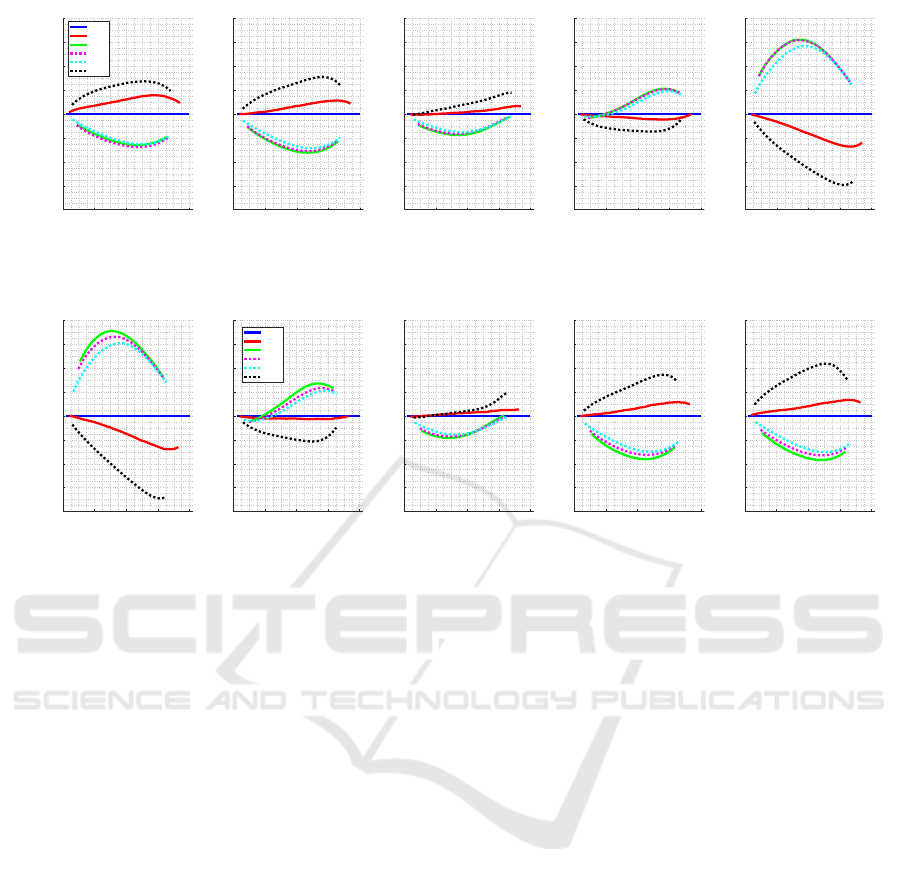
Combining Stop Criteria. Because each stop crite-
rion method present different characteristics, we may
consider combining two or more methods to present
a better performance. (Babcock and Weiss, 2009)
and Morris et al. (2020) consider ad hoc combination.
Here, we consider an optimization based on our pro-
posed trade-off curve.
Consider again the partition of examinees in five
range. Figures 10 and 11 show the RMSE of each
stop-criterion method in each range for EAP and ML
estimations, respectively. We choose the class of
item bank based on normal distribution and shift level
equal -1; this was the class where we observe greater
difference through ranges, so that none method dom-
inated the others.
We consider two combination of stop criteria: ora-
cle and estimated. In the case of oracle is a unrealistic
case, when the examiner knows the range where the
examinee comes from and can choose the best stop
criteria for each examinee; therefore, improvement is
guaranteed. In the case of estimated, the examiner
estimates the trait of the examinee based on answer
to applied items and choose the stop criterion online,
changing when it is necessary.
Figure 10 and 11 show the mean result of both
mixed stop criteria, using EAP and ML in the estima-
tion, based on the actual ability (red dots) and esti-
mated ability (green dots).
The results shows that when we differentiate the
individuals, that is, we consider the trait levels sepa-
rately, it is possible to improve the RMSE by combin-
ing the stop criteria. The improvement is more salient
Comprehensive Empirical Analysis of Stop Criteria in Computerized Adaptive Testing
55

10 15 20 25 30 35 40 45 50
Mean CAT Length
0.24
0.26
0.28
0.3
0.32
0.34
0.36
Mean RMSE
Full Population
MI
CT
SE
VAP
VVAP
FL
Mixed Oracle
Mixed Estimated
10 15 20 25 30 35 40 45 50
Mean CAT Length
0.2
0.25
0.3
0.35
Mean RMSE
1st range
10 15 20 25 30 35 40 45 50
Mean CAT Length
0.18
0.2
0.22
0.24
0.26
0.28
0.3
Mean RMSE
2nd range
10 15 20 25 30 35 40 45 50
Mean CAT Length
0.2
0.22
0.24
0.26
0.28
0.3
0.32
Mean RMSE
3rd range
10 15 20 25 30 35 40 45 50
Mean CAT Length
0.22
0.24
0.26
0.28
0.3
0.32
0.34
Mean RMSE
4th range
10 15 20 25 30 35 40 45 50
Mean CAT Length
0.34
0.36
0.38
0.4
0.42
0.44
0.46
Mean RMSE
5th range
Figure 10: Mean of all stop criteria mixed using EAP in estimating ability.
10 15 20 25 30 35 40 45 50
Mean CAT Length
0.26
0.28
0.3
0.32
0.34
0.36
0.38
0.4
Mean RMSE
Full Population
MI
CT
SE
VAP
VVAP
FL
Mixed Oracle
Mixed Estimated
10 15 20 25 30 35 40 45 50
Mean CAT Length
0.2
0.22
0.24
0.26
0.28
0.3
0.32
0.34
0.36
0.38
0.4
Mean RMSE
1st range
10 15 20 25 30 35 40 45 50
Mean CAT Length
0.18
0.2
0.22
0.24
0.26
0.28
0.3
0.32
0.34
Mean RMSE
2nd range
10 15 20 25 30 35 40 45 50
Mean CAT Length
0.2
0.25
0.3
0.35
Mean RMSE
3rd range
10 15 20 25 30 35 40 45 50
Mean CAT Length
0.25
0.3
0.35
0.4
Mean RMSE
4th range
10 15 20 25 30 35 40 45 50
Mean CAT Length
0.39
0.4
0.41
0.42
0.43
0.44
0.45
0.46
0.47
Mean RMSE
5th range
Figure 11: Mean of all stop criteria mixed using ML in estimating ability.
when considering ML estimation.
Although the method based on oracle shows some
improvement, the improvement is not large, even
when we consider the best class of item bank to
present such a improvement. On the other side, the
method based on estimated does not even shows im-
provement with EAP estimation, which may shows
that estimation is too fuzzy to be used as a guide to
condition stop criterion or selection criterion.
CSEDU 2021 - 13th International Conference on Computer Supported Education
56

5 DISCUSSION AND
CONCLUSION
The use of CATs has become increasingly popular, es-
pecially during the covid pandemic, where due to the
need for social distance the tests are done via com-
puter. Given this, we emphasize the importance of
discussing the best stopping criteria for fairer exams,
as these directly influence the final result.
The proposed stop criterion, VVAP, presents a
similar performance to the majority of other crite-
ria, however it is worse when compared to the FL
for having a greater standard deviation in the number
of questions. This is also an advantage of the Fixed
Length criterion for all the other criteria considered.
Although many works use mixed stop criteria, it
was observed that it do not seem to improve the mean
RMSE when the full population is considered.
We conclude in favor of the FI criterion, as long as
it can be tuned to the item bank at hand. The FL shows
a competitive precision-efficiency trade-off curve in
every scenario while presenting zero variance in test
length.
The threshold definition methods presented were
important to compare in a fair way all the criteria on
every item bank.
The limitation of the current research is to fix only
the ML3 of the IRT for the calculation of the correct
score probability and to make tests only in simulated
item banks. Future works can be developed using
other models of IRT and using actual item data.
The research was very important for being able to
compare the stop criteria in several scenarios: using
the ML and EAP method, several distributions for the
parameter b of the IRT model, with and without shifts,
and to analyze a large number of trade-offs.
REFERENCES
Babcock, B. and Weiss, D. (2009). Termination criteria in
computerized adaptive tests: Variable-length cats are not
biased. In Proceedings of the 2009 GMAC conference on
computerized adaptive testing, volume 14.
Birnbaum, A. L. (1968). Some latent trait models and their
use in inferring an examinee’s ability. Statistical theories
of mental test scores.
Chang, H.-H. and Ying, Z. (1996). A global information
approach to computerized adaptive testing. Applied Psy-
chological Measurement, 20(3):213–229.
de Andrade, D. F., Tavares, H. R., and da Cunha Valle,
R. (2000). Teoria da resposta ao item: conceitos e
aplicac¸
˜
oes. ABE, S
˜
ao Paulo.
Hambleton, R. K. and Swaminathan, H. (2013). Item re-
sponse theory: Principles and applications. Springer
Science & Business Media.
Kreitzberg, C. B., Stocking, M. L., and Swanson, L. (1978).
Computerized adaptive testing: Principles and direc-
tions. Computers & Education, 2(4):319–329.
Lord, F. M. (1980). Applications of item response theory to
practical testing problems. Routledge.
Morris, S. B., Bass, M., Howard, E., and Neapolitan, R. E.
(2020). Stopping rules for computer adaptive testing
when item banks have nonuniform information. Inter-
national journal of testing, 20(2):146–168.
Sari, H. I. and Raborn, A. (2018). What information works
best?: A comparison of routing methods. Applied psy-
chological measurement, 42(6):499–515.
Segall, D. O. (2005). Computerized adaptive testing. Ency-
clopedia of social measurement, 1:429–438.
Spenassato, D., Bornia, A., and Tezza, R. (2015). Comput-
erized adaptive testing: A review of research and tech-
nical characteristics. IEEE Latin America Transactions,
13(12):3890–3898.
Stafford, R. E., Runyon, C. R., Casabianca, J. M., and
Dodd, B. G. (2019). Comparing computer adaptive test-
ing stopping rules under the generalized partial-credit
model. Behavior research methods, 51(3):1305–1320.
van der Linden, W. J. (1998). Bayesian item selection crite-
ria for adaptive testing. Psychometrika, 63(2):201–216.
van der Linden, W. J. and Glas, C. A. (2000). Computerized
Adaptive Testing: Theory and Practice. Springer Science
& Business Media, Boston, MA.
Veerkamp, W. J. and Berger, M. P. (1997). Some new item
selection criteria for adaptive testing. Journal of Educa-
tional and Behavioral Statistics, 22(2):203–226.
Wainer, H., Dorans, N. J., Flaugher, R., Green, B. F., and
Mislevy, R. J. (2000). Computerized adaptive testing: A
primer. Routledge.
Wang, C., Chang, H.-H., and Huebner, A. (2011). Restric-
tive stochastic item selection methods in cognitive diag-
nostic computerized adaptive testing. Journal of Educa-
tional Measurement, 48(3):255–273.
Comprehensive Empirical Analysis of Stop Criteria in Computerized Adaptive Testing
57

APPENDIX
10 15 20 25 30
CAT Length
-5
0
5
10
∆ RMSE
× 10
-3
Uniform, Shift=-1
FI
MEPV
KL
KLP
MLWI
MPWI
10 15 20 25 30
CAT Length
-5
0
5
10
∆ RMSE
× 10
-3
Uniform, Shift=0
10 15 20 25 30
CAT Length
-5
0
5
10
∆ RMSE
× 10
-3
Uniform, Shift=1
10 15 20 25 30
CAT Length
-5
0
5
10
∆ RMSE
× 10
-3
Peak, Shift=-1
10 15 20 25 30
CAT Length
-5
0
5
10
∆ RMSE
× 10
-3
Peak, Shift=0
10 15 20 25 30
CAT Length
-5
0
5
10
∆ RMSE
× 10
-3
Peak, Shift=1
10 15 20 25 30
CAT Length
-5
0
5
10
∆ RMSE
× 10
-3
Normal, Shift=-1
10 15 20 25 30
CAT Length
-5
0
5
10
∆ RMSE
× 10
-3
Normal, Shift=0
10 15 20 25 30
CAT Length
-5
0
5
10
∆ RMSE
× 10
-3
Normal, Shift=1
Figure 12: Comparison of item selection criteria using FL as a stop criterion and EAP for estimation.
10 15 20 25 30
CAT Length
-0.03
-0.02
-0.01
0
0.01
∆ RMSE
Uniform, Shift=-1
FI
MEPV
KL
KLP
MLWI
MPWI
10 15 20 25 30
CAT Length
-0.03
-0.02
-0.01
0
0.01
∆ RMSE
Uniform, Shift=0
10 15 20 25 30
CAT Length
-0.03
-0.02
-0.01
0
0.01
∆ RMSE
Uniform, Shift=1
10 15 20 25 30
CAT Length
-0.03
-0.02
-0.01
0
0.01
∆ RMSE
Peak, Shift=-1
10 15 20 25 30
CAT Length
-0.03
-0.02
-0.01
0
0.01
∆ RMSE
Peak, Shift=0
10 15 20 25 30
CAT Length
-0.03
-0.02
-0.01
0
0.01
∆ RMSE
Peak, Shift=1
10 15 20 25 30
CAT Length
-0.03
-0.02
-0.01
0
0.01
∆ RMSE
Normal, Shift=-1
10 15 20 25 30
CAT Length
-0.03
-0.02
-0.01
0
0.01
∆ RMSE
Normal, Shift=0
10 15 20 25 30
CAT Length
-0.03
-0.02
-0.01
0
0.01
∆ RMSE
Normal, Shift=1
Figure 13: Comparison of item selection criteria using FL as a stop criterion and ML for estimation.
CSEDU 2021 - 13th International Conference on Computer Supported Education
58

10 15 20 25 30 35 40 45 50
CAT Length
-0.005
0
0.005
0.01
0.015
0.02
0.025
∆ RMSE
Uniform, Shift=-1
FL
CT
SE
VAP
VVAP
MI
10 15 20 25 30 35 40 45 50
CAT Length
-0.005
0
0.005
0.01
0.015
0.02
0.025
∆ RMSE
Uniform, Shift=0
10 15 20 25 30 35 40 45 50
CAT Length
-0.005
0
0.005
0.01
0.015
0.02
0.025
∆ RMSE
Uniform, Shift=1
10 15 20 25 30 35 40 45 50
CAT Length
-0.005
0
0.005
0.01
0.015
0.02
0.025
∆ RMSE
Peak, Shift=-1
10 15 20 25 30 35 40 45 50
CAT Length
-0.005
0
0.005
0.01
0.015
0.02
0.025
∆ RMSE
Peak, Shift=0
10 15 20 25 30 35 40 45 50
CAT Length
-0.005
0
0.005
0.01
0.015
0.02
0.025
∆ RMSE
Peak, Shift=1
10 15 20 25 30 35 40 45 50
CAT Length
-0.005
0
0.005
0.01
0.015
0.02
0.025
∆ RMSE
Normal, Shift=-1
10 15 20 25 30 35 40 45 50
CAT Length
-0.005
0
0.005
0.01
0.015
0.02
0.025
∆ RMSE
Normal, Shift=0
10 15 20 25 30 35 40 45 50
CAT Length
-0.005
0
0.005
0.01
0.015
0.02
0.025
∆ RMSE
Normal, Shift=1
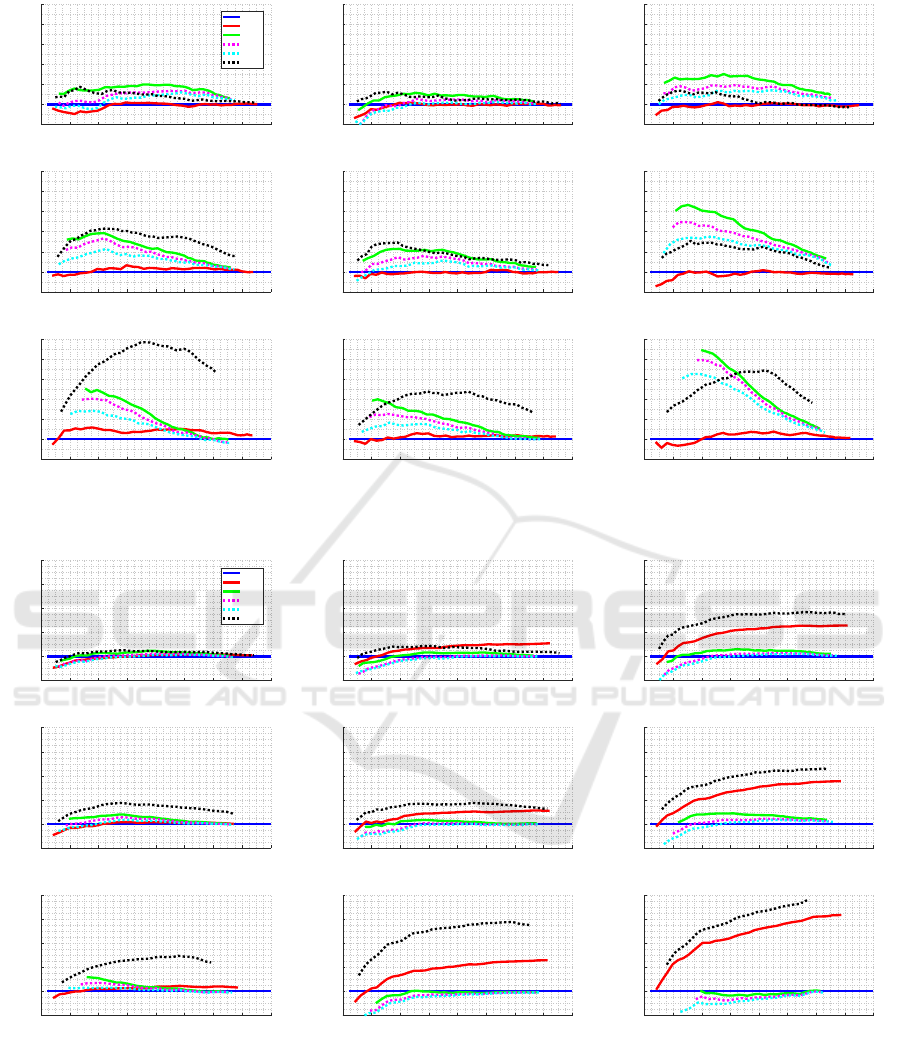
Figure 14: Comparison of stop criteria using FI as an item selection criterion and EAP for estimation.
10 15 20 25 30 35 40 45 50
CAT Length
-0.02
0
0.02
0.04
0.06
0.08
∆ RMSE
Uniform, Shift=-1
FL
CT
SE
VAP
VVAP
MI
10 15 20 25 30 35 40 45 50
CAT Length
-0.02
0
0.02
0.04
0.06
0.08
∆ RMSE
Uniform, Shift=0
10 15 20 25 30 35 40 45 50
CAT Length
-0.02
0
0.02
0.04
0.06
0.08
∆ RMSE
Uniform, Shift=1
10 15 20 25 30 35 40 45 50
CAT Length
-0.02
0
0.02
0.04
0.06
0.08
∆ RMSE
Peak, Shift=-1
10 15 20 25 30 35 40 45 50
CAT Length
-0.02
0
0.02
0.04
0.06
0.08
∆ RMSE
Peak, Shift=0
10 15 20 25 30 35 40 45 50
CAT Length
-0.02
0
0.02
0.04
0.06
0.08
∆ RMSE
Peak, Shift=1
10 15 20 25 30 35 40 45 50
CAT Length
-0.02
0
0.02
0.04
0.06
0.08
∆ RMSE
Normal, Shift=-1
10 15 20 25 30 35 40 45 50
CAT Length
-0.02
0
0.02
0.04
0.06
0.08
∆ RMSE
Normal, Shift=0
10 15 20 25 30 35 40 45 50
CAT Length
-0.02
0
0.02
0.04
0.06
0.08
∆ RMSE
Normal, Shift=1
Figure 15: Comparison of stop criteria using FI as an item selection criterion and ML for estimation.
Comprehensive Empirical Analysis of Stop Criteria in Computerized Adaptive Testing
59