Deep Learning Classifiers for Automated Driving: Quantifying the
Trained DNN Model’s Vulnerability to Misclassification
Himanshu Agarwal
1,2
, Rafal Dorociak
1
and Achim Rettberg
2,3
1
HELLA GmbH & Co. KGaA, Lippstadt, Germany
2
Department of Computing Science, Carl von Ossietzky University Oldenburg, Germany
3
University of Applied Sciences Hamm-Lippstadt, Lippstadt, Germany
Keywords:
Image Classification, Deep Learning, Deep Neural Network, Vulnerability to Misclassification, Automated
Driving.
Abstract:
The perception-based tasks in automated driving depend greatly on deep neural networks (DNNs). In context
of image classification, the identification of the critical pairs of the target classes that make the DNN highly
vulnerable to misclassification can serve as a preliminary step before implementing the appropriate measures
for improving the robustness of the DNNs or the classification functionality. In this paper, we propose that
the DNN’s vulnerability to misclassifying an input image into a particular incorrect class can be quantified
by evaluating the similarity learnt by the trained model between the true class and the incorrect class. We
also present the criteria to rank the DNN model’s vulnerability to a particular misclassification as either low,
moderate or high. To argue for the validity of our proposal, we conduct an empirical assessment on DNN-
based traffic sign classification. We show that upon evaluating the DNN model, most of the images for which
it yields an erroneous prediction experience the misclassifications to which its vulnerability was ranked as
high. Furthermore, we also validate empirically that all those possible misclassifications to which the DNN
model’s vulnerability is ranked as high are difficult to deal with or control, as compared to the other possible
misclassifications.
1 INTRODUCTION
In the recent years, the advancements in the field of
autonomous driving have been reinforced with the
progress in the techniques of artificial intelligence,
especially deep learning. A survey of the current
state-of-the-art deep learning technologies, e.g., deep
convolutional neural networks, deep reinforcement
learning, etc., has been presented in Grigorescu et al.
(2019). The deep convolutional neural networks have
led to various breakthrough contributions in object
detection and image classification tasks, such as in
Krizhevsky et al. (2012) and Sermanet et al. (2014).
In context of autonomous driving, deep learning plays
a major role in perception-based tasks such as pedes-
trian detection (Ouyang et al., 2017), traffic sign de-
tection (Zhu et al., 2016), etc. One of the challenges in
safe automated driving is related to the robustness of
the artificial intelligence or deep learning techniques
(Muhammad et al., 2020). In context of tasks related
to image classification, it must be ensured that the
deep neural networks (DNNs) are not just accurate
but also robust against the perturbations that a vehicle
might encounter during its operation. The perturba-
tions, for instance, can be random noise in the input
images or even shift in brightness, contrast, etc. These
perturbations can influence the DNN’s decision sig-
nificantly and aggravate the chances of misclassifying
an input image into an incorrect class that is highly
similar with respect to the true class. The questions
which need to be addressed are as follows:
• Since an image X
X
X belonging to the true class k
1
can be misclassified into any of the remaining tar-
get classes, how can we rank all these possible
misclassifications on the basis of how vulnerable
is the DNN model to each of them individually?
• If the misclassification from a true class k
1
into
an another class k
2
(6= k
1
) is ranked to be offering
a high vulnerability, do the perturbations in the
images exploit this vulnerability and give rise to a
higher misclassification rate from k
1
into k
2
?
Such investigations can help in determining the set
of critical misclassifications that need laborious miti-
Agarwal, H., Dorociak, R. and Rettberg, A.
Deep Learning Classifiers for Automated Driving: Quantifying the Trained DNN Model’s Vulnerability to Misclassification.
DOI: 10.5220/0010481302110222
In Proceedings of the 7th International Conference on Vehicle Technology and Intelligent Transport Systems (VEHITS 2021), pages 211-222
ISBN: 978-989-758-513-5
Copyright
c
 2021 by SCITEPRESS – Science and Technology Publications, Lda. All rights reserved
211

gation efforts to enhance the robustness of the classi-
fication function.
Our contributions in this paper are listed below:
• We propose an approach to estimate the trained
DNN model’s vulnerability to a particular mis-
classification. Along with it, we propose the crite-
ria to categorise the DNN model’s vulnerability to
a particular misclassification into one of the three
levels: low, moderate or high.
• We further argue that the ease with which the rate
of a particular misclassification can be kept un-
der control depends on the estimated value of the
DNN model’s vulnerability to it. In other words,
we highlight that it is easier to control those mis-
classifications to which the model is estimated to
be lowly vulnerable, as compared to the misclassi-
fications to which it is estimated to be highly vul-
nerable. We validate our arguments empirically.
The practical examples and the corresponding ex-
perimentation
1
conducted in context of the above-
mentioned contributions have been extensively dis-
cussed in the paper. The remainder of the paper is
organized as follows. In Section 2, we present a brief
background to discuss the rationale behind our pro-
posed approach of estimating the DNN’s vulnerabil-
ity to a particular misclassification. In Section 3, we
present a detailed description of the approach, and an
experimental analysis in context of traffic sign classi-
fication. Section 4 addresses the second part of our
contributions, i.e., an empirical investigation to show
that the set of misclassifications to which the DNN
model is ranked to be highly vulnerable are rather
difficult to manage, even after the implementation of
the measures to control the misclassification rate. Fi-
nally, Section 5 presents a conclusion along with a
brief overview on the possible future directions.
2 BACKGROUND
In context of image classification, the objective is to
ensure that a classifier is able to correctly distinguish
between the target classes. In Tian et al. (2020), for
instance, the authors assess the classifier model’s abil-
ity to distinguish between any two classes by comput-
ing the confusion score. This score is based on mea-
suring the euclidean distance between the neuron ac-
tivation probability vectors corresponding to the two
1
For the experimentation, the libraries: Numpy (Harris
et al., 2020), Keras (Chollet et al., 2015), SciPy (Virta-
nen et al., 2020), Scikit-learn (Pedregosa et al., 2011) and
Matplotlib (Hunter, 2007) were used along with some of
the other standard Python libraries and their functions.
classes. Such analyses are usually performed by eval-
uating the trained model against a set of independent
(test) images. However, such evaluations against a set
of test images are not sufficient to realize the classi-
fier’s ability to distinguish between the classes (since
the completeness of the test data serves as a major
challenge). As an additional assessment, the critical
misclassifications corresponding to the DNN model
can be identified by determining the set of possible
misclassifications to which the model is highly vul-
nerable. In Agarwal et al. (2021), it has been argued
that the classifier’s vulnerability to a particular mis-
classification (let us say, from the true class k
1
into
an incorrect class k
2
or vice versa) can be assessed in
terms of the similarity between the dominant visual
characteristics of the corresponding two classes (i.e.,
k
1
and k
2
). For instance, the dominant visual charac-
teristics in the traffic signs are shape and color (Gao
et al., 2006). By evaluating the overlap in terms of (a)
the shape of the traffic sign board, and (b) the color
combination of the border and the background, the
similarity between any two traffic sign classes can be
analysed a priori (Agarwal et al., 2021). The obtained
measure of similarity between the classes k
1
and k
2
is
recognized as a measure of the classifier’s vulnerabil-
ity to misclassifying an input image belonging to the
class k
1
into the class k
2
or vice versa. Higher simi-
larity between the two classes is considered to induce
higher vulnerability to the corresponding misclassifi-
cation.
We illustrate it further with an example. In this re-
gard, we trained a DNN to classify the different traf-
fic signs from the German Traffic Sign Recognition
Benchmark (GTSRB) dataset (Stallkamp et al., 2012).
Mathematically, we represent the DNN (classifier)
model as f : X
X
X ∈ R
(48×48×3)
−→ ˆy ∈ {1,2,...,43},
where ˆy is the predicted class for the input image X
X
X.
The hyperparameters and the training details related
to it are provided in Appendix A. From the set of
10000 test images, we choose 2207 images which be-
long to the danger sign type. We determine the per-
centage of these images that the DNN model f mis-
classifies into: (a) another danger sign, (b) a speed
limit or a prohibitory sign, (c) a derestriction sign,
and (d) a mandatory sign. The results are graphically
presented in Figure 1. We first consider the results
plotted for the GTSRB original test images (i.e., the
test images without any perturbations deliberately en-
forced by us). We observe a higher rate of misclassi-
fication of a danger sign into another danger sign, as
compared to the other misclassifications. All the traf-
fic signs that belong to the danger sign type have high
similarity due to their two dominant visual character-
istics being the same. This can perhaps be a potential
VEHITS 2021 - 7th International Conference on Vehicle Technology and Intelligent Transport Systems
212

0 2 4 6 8 10 12
1
2
3
4
Figure 1: Graph showing the percentage of the danger sign
images in the test dataset that were misclassified into: an-
other danger sign, speed limit or prohibitory sign, derestric-
tion sign, and mandatory sign.
source of the higher rate of misclassification of a dan-
ger sign into another danger sign, as observed in Fig-
ure 1. It can also be observed that some common per-
turbations (e.g., contrast change, gaussian blur, etc.)
enforced by us on the GTSRB original test images
further aggravate the DNN’s susceptibility to misclas-
sification of a danger sign into another danger sign.
This indicates that the DNNs used for image classi-
fication are rather more susceptible or vulnerable to
misclassification of an input image into the classes
that have stronger visual similarity with the true class.
This estimation of similarity depending on the
chosen predominant visual characteristics can facil-
itate the planning of the pre-training activities. For
instance, it can help the experts in choosing a suit-
able configuration of the DNN architecture or tailor-
ing the DNN-based strategy appropriately in a manner
that has the potential to minimize those misclassifi-
cations wherein the true class and the incorrect class
are highly similar in terms of their visual appearance.
However, it must be noted that the visual characteris-
tics considered in the abovementioned a priori anal-
ysis of similarity may not always necessarily be the
features that actually influence the decision of the
classifier (Ribeiro et al., 2016). Thus, the similar-
ity perceived by humans between any two classes is
not necessarily the similarity that will be learnt by the
DNN model via training. As an extension to this con-
cept, unlike the approach discussed in Agarwal et al.
(2021), in this paper, we propose to estimate the DNN
model’s vulnerability to misclassification from class
k
1
into class k
2
by measuring the similarity learnt by
the trained model between the classes k
1
and k
2
. In
our approach of measuring the class similarity learnt
by the DNN model, we use the images from the train-
ing dataset itself. Hence, by virtue of this vulnera-
bility estimation, we identify the set of critical mis-
classifications without actually evaluating the trained
model against any independent or seperate set of the
images (i.e., test data). The approach has been elabo-
rated in Section 3.
3 VULNERABILITY TO
MISCLASSIFICATION
Let us assume the DNN (classifier) is trained for
K number of target classes. A class k ∈ K =
{1,2,....,K} can be misclassified into any of the re-
maining (K − 1) classes. Therefore, the set of mis-
classifications that it can incur is represented as:
M = { (k
a
,k
b
) | k
a
6= k
b
, k
a
∈ K , k
b
∈ K }, (1)
where k
a
and k
b
represent the true class and the incor-
rect class, respectively. The total number of misclas-
sifications that are possible is |M | = K(K − 1).
The DNN’s vulnerability to a particular misclassi-
fication, let us say, (k
a
,k
b
), is determined by evaluat-
ing the similarity between the two classes k
a
and k
b
.
Followed by this, the categorisation criteria is imple-
mented in order to identify the set of possible misclas-
sifications to which the DNN model is highly vulner-
able. The approach has been discussed in this section,
along with an experimental analysis.
3.1 Similarity between the Classes
In order to measure the class similarity learnt by the
trained model, the approach discussed in Agarwal
et al. (2020) is used. The trained DNN model pre-
dicts the logits z
z
z
k
= [z
1
,z
2
,....,z
K
] for an input im-
age belonging to a class k ∈ K . The predicted logits
z
z
z
k
is then modelled as a multivariate normal distri-
bution N
k
. Mathematically, z
z
z
k
∼ N
k
(µ
µ
µ
k
,Σ
Σ
Σ
k
), where
µ
µ
µ
k
and Σ
Σ
Σ
k
represent the K × 1 mean vector and the
K × K covariance matrix of the distribution N
k
. The
similarity between any two classes is determined by
calculating the Bhattacharyya distance between their
corresponding modelled multivariate normal distribu-
tions. Let us consider the classes k
a
and k
b
here. The
Bhattacharyya distance d
k
a
,k
b
between N
k
a
(µ
µ
µ
k
a
,Σ
Σ
Σ
k
a
)
and N
k
b
(µ
µ
µ
k
b
,Σ
Σ
Σ
k
b
) is determined using Equation 2
(Kashyap, 2019).
d
k
a
,k
b
=
1
8
(µ
µ
µ
k
a
− µ
µ
µ
k
b
)
T
Σ
Σ
Σ
−1
avg
(µ
µ
µ
k
a
− µ
µ
µ
k
b
)
+
1
2
ln
|Σ
Σ
Σ
avg
|
p
|Σ
Σ
Σ
k
a
||Σ
Σ
Σ
k
b
|
!
, (2)
Deep Learning Classifiers for Automated Driving: Quantifying the Trained DNN Model’s Vulnerability to Misclassification
213

where
Σ
Σ
Σ
avg
=
1
2
(Σ
Σ
Σ
k
a
+ Σ
Σ
Σ
k
b
). (3)
The similarity between the classes k
a
and k
b
will
be inversely proportional to the computed value of the
Bhattacharyya distance d
k
a
,k
b
. It must be noted that
the Bhattacharyya distance computed above is sym-
metric, i.e., d
k
a
,k
b
= d
k
b
,k
a
.
3.2 Estimation of Vulnerability
Using the approach discussed in Section 3.1, we can
compute the value of d to assess the similarity of a
class k ∈ K with every other class in K \ {k}. Since
the number of target classes is K, we will have a total
K(K − 1) values of the Bhattacharyya distances. We
accumulate all these obtained values in a set D, as
shown below:
D = { d
k
a
,k
b
| k
a
6= k
b
, k
a
∈ K , k
b
∈ K }. (4)
Among all these K(K − 1) values, let us assume
that the maximum value is observed to be d
max
, i.e.,
d
max
= max (D). (5)
Now, we represent the DNN model’s vulnerability
to the misclassification (k
a
,k
b
) as:
v(k
a
,k
b
) = 1 −
d
k
a
,k
b
d
max
. (6)
Note that v(k
a
,k
b
)∈[0,1) and v(k
a
,k
b
)=v(k
b
,k
a
).
Since v(k
a
,k
b
)=1 is possible only if k
a
=k
b
(which
does not represent the case of misclassification),
therefore, the value of 1 is excluded from the speci-
fied range of v(k
a
,k
b
). The value of v(k
a
,k
b
) closer to
1 indicates higher vulnerability to the corresponding
misclassification (k
a
,k
b
).
3.3 Categorisation Criteria
Using the approach discussed above, we can acquire
the model’s vulnerability values corresponding to all
the K(K − 1) possible misclassifications. We collect
all these obtained values in a set V , as shown below:
V = { v(k
a
,k
b
) | (k
a
,k
b
) ∈ M }. (7)
We will now categorise the model’s vulnerability
to a particular misclassification into one of the levels:
low, moderate or high, using certain statistical mea-
sures, as discussed below.
To the misclassification (k
a
,k
b
), the DNN model
will be considered to have:
• low vulnerability if 0 ≤ v(k
a
,k
b
) < p
25
,
• moderate vulnerability if p
25
≤ v(k
a
,k
b
) < p
75
,
and
• high vulnerability if p
75
≤ v(k
a
,k
b
) < 1,
where p
25
and p
75
are the 25
th
and the 75
th
percentile
of the values in the set V , respectively.
The set of the misclassifications to which the DNN
model’s vulnerability is ranked as low, moderate and
high are denoted as M
low
,M
moderate
and M
high
, re-
spectively. They are mathematically represented as:
M
low
= { (k
a
,k
b
) ∈ M | 0 ≤ v(k
a
,k
b
) < p
25
},
(8)
M
moderate
= { (k
a
,k
b
) ∈ M | p
25
≤ v(k
a
,k
b
) < p
75
},
(9)
M
high
= { (k
a
,k
b
) ∈ M | p
75
≤ v(k
a
,k
b
) < 1 }.
(10)
Note that: (i) M
low
∩ M
moderate
=
/
0, (ii)
M
moderate
∩M
high
=
/
0, (iii) M
low
∩M
high
=
/
0, and (iv)
M
low
∪ M
moderate
∪ M
high
= M .
In order to support the validity of this proposed
criteria of categorising the DNN model’s vulnerabil-
ity, we conducted an experimental analysis, which has
been discussed in Section 3.4.
3.4 Experimental Analysis
3.4.1 DNN Training
We conducted our experiment for the classification of
the traffic signs from the GTSRB dataset. The DNN
model used here in this experimental analysis is the
same model f : X
X
X ∈ R
(48×48×3)
→ ˆy ∈ {1, 2, ...,43},
which was trained for the illustration of the example
presented in Section 2. A brief summary of the DNN
architecture and the associated details related to it’s
training are provided in Appendix A. Since the total
number of target traffic sign classes is K = 43, the
number of possible misclassifications is |M | = 43 ×
42 = 1806.
3.4.2 Vulnerability to Misclassification
We first determined the similarity learnt by the DNN
model f between all the 43 target traffic sign classes,
using the approach discussed in Section 3.1. Note that
in order to model the logits z
z
z
k
as a multivariate nor-
mal distribution, the samples of the predicted logits z
z
z
k
were collected for all the images in the training data
that belong to the class k. Followed by the measure-
ment of similarity between the classes, we determined
the model’s vulnerability (v) to each of the 1806 pos-
sible misclassifications, as discussed in Section 3.2.
The distribution of the obtained 1806 values of v is il-
lustrated as a histogram in Figure 2. The 25
th
and the
75
th
percentile of the distribution are p
25
= 0.4354
and p
75
= 0.6455, respectively.
VEHITS 2021 - 7th International Conference on Vehicle Technology and Intelligent Transport Systems
214

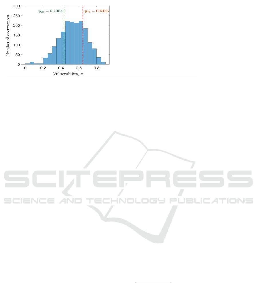
Figure 2: Distribution of the trained DNN model’s esti-
mated vulnerability (v) to the 1806 possible misclassifica-
tions among the 43 traffic sign classes. The terms p
25
and
p
75
denote the 25
th
and the 75
th
percentile of the distribu-
tion, respectively.
3.4.3 Evaluation
The trained model f was evaluated on τ = 10000 GT-
SRB test images. We represent the set of these test
images as X
test
= {X
X
X
1
,X
X
X
2
,...,X
X
X
τ
}. An accuracy of
96.12% was observed. Alternatively, it can be said
that the model misclassifies ρ = 388 traffic sign im-
ages from X
test
. Let us denote the set of the misclas-
sified images as X
m
= {X
X
X
m
1
,X
X
X
m
2
,...,X
X
X
m
ρ
}, such that
X
m
⊂ X
test
. The corresponding misclassifications ex-
perienced by the model for the images in X
m
are put
together in the set Ψ
m
, as shown below:
Ψ
m
={(y
m
1
, ˆy
m
1
),(y
m
2
, ˆy
m
2
),...,(y
m
ρ
, ˆy
m
ρ
)}, (11)
where the ordered pair (y
m
i
, ˆy
m
i
) ∈ M signifies that
for the image X
X
X
m
i
∈ X
m
, the actual class is y
m
i
; how-
ever, the model f predicts it as a class ˆy
m
i
∈ K \{y
m
i
}.
Out of all the images in X
m
, the number of images
for which the corresponding misclassifications in Ψ
m
were ranked to be offering the model f , based on our
proposed criteria, a:
(a) Low vulnerability equals:
n
low
=
ρ
∑
i=1
[0 ≤ v(y
m
i
, ˆy
m
i
) < p
25
], (12)
(b) Moderate vulnerability equals:
n
moderate
=
ρ
∑
i=1
[p
25
≤ v(y
m
i
, ˆy
m
i
) < p
75
], (13)
(c) High vulnerability equals:
n
high
=
ρ
∑
i=1
[p
75
≤ v(y
m
i
, ˆy
m
i
) < 1], (14)
where [...] in (12), (13) and (14) denote the Iverson
brackets, and v(y
m
i
, ˆy
m
i
) denotes the model’s vulner-
ability to the misclassification (y
m
i
, ˆy
m
i
). Note that:
n
low
+ n
moderate
+ n
high
= ρ. (15)
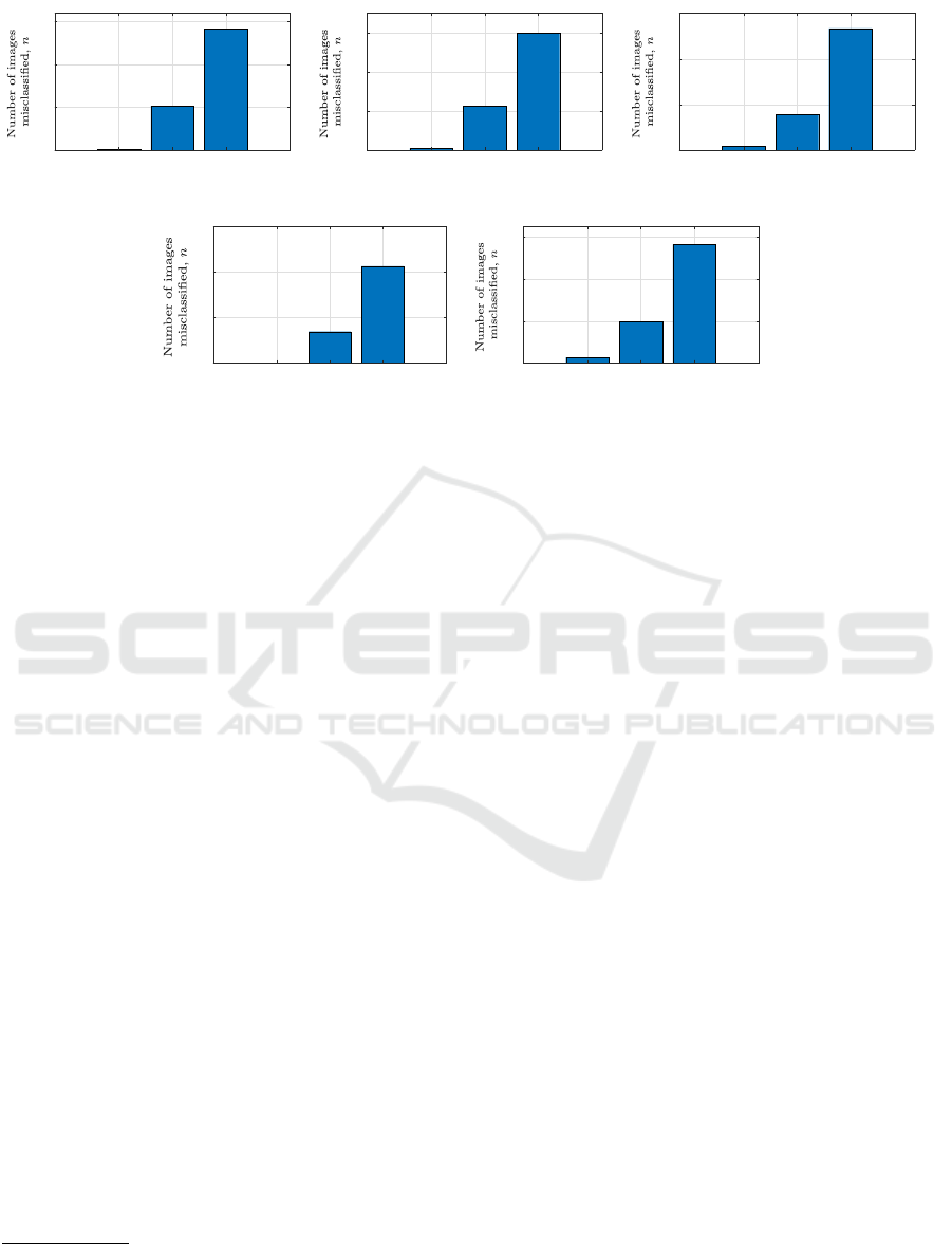
For X
test
, using the trained classifier model f , we
got the values of n
low
, n
moderate
and n
high
as 1, 103 and
284, respectively. This has been graphically presented
in Figure 3a. It can be deduced that:
n
high
> n
moderate
> n
low
, (16)
which implies, the model is most likely to incur
those misclassifications to which it’s vulnerability
was ranked to be high. To further validate this, we
continue our analysis using the perturbed test images.
These perturbations are: change in contrast
2
, change
in brightness
3
, gaussian blur
4
and gaussian noise
5
.
We apply these perturbations seperately to every im-
age X
X
X
j
in X
test
, j = 1 to τ. Hence, we have four dif-
ferent sets of perturbed test images, i.e., X
∆contrast
,
X
∆brightness
, X
∆blur
and X
∆noise
. The corresponding
obtained values of n
low
,n
moderate
and n
high
are graphi-
cally presented in Figure 3b - 3e. It can be observed
that the condition in (16) holds true for the analysis
associated with the perturbed test images as well.
The criteria proposed for categorisation seems co-
herent or convincing when analysed experimentally
on a classification problem, as it does helps in deter-
mining the set of critical misclassifications, i.e., the
set of misclassifications which the DNN model can
most likely incur. Hence, the concept of using the
class similarity learnt by the model for quantifying
it’s vulnerability to every possible misclassification
appears to be reasonable.
4 Further Empirical Investigation
4.1 Concept and Purpose
One of the ways to minimize the possibility of an
erroneous prediction or a misclassification incurred
by a DNN model is to integrate a mechanism that
can provide the classification functionality an alter-
native to not yield any decision in case of lack of cer-
tainty. For this purpose, in addition to the classifier
2
every pixel p(r,s,t) ∈ [0,1] of a test image X
X
X
j
undergoes
a transformation: p(r,s,t) → γ p(r,s,t), using a randomly
chosen γ ∈ [1, 3].
3
every pixel p(r,s,t) ∈ [0, 1] of a test image X
X
X
j
undergoes a
transformation: p(r, s,t) → p(r,s,t) + δ, using a randomly
chosen δ ∈ [0, 0.4].
4
function in the OpenCV library (https://github.com/
opencv/opencv). To perturb a test image X
X
X
j
, we choose
randomly a kernel size η ∈ {3, 5,7}, and the standard de-
viation σ ∈ [0.5, 1.5] along both x and y directions.
5
adding to a test image X
X
X
j
a random normal gaussian noise
with a mean µ = 0 and a randomly chosen standard devia-
tion σ ∈ [0.01, 0.1].
Deep Learning Classifiers for Automated Driving: Quantifying the Trained DNN Model’s Vulnerability to Misclassification
215

1
103
284
Low Moderate High
0
100
200
300
(a) Original test images
4
112
299
Low Moderate High
0
100
200
300
(b) Test images with contrast change
15
156
533
Low Moderate High
0
200
400
600
(c) Test images with brightness change
2
138
425
Low Moderate High
0
200
400
600
(d) Test images with gaussian blur
27
197
564
Low Moderate High
0
200
400
600
(e) Test images with gaussian noise
Figure 3: Graphs showing the values of n
low
, n
moderate
and n
high
, obtained when the trained DNN model was evaluated for
different sets of the test images: (a) X
test
, (b) X
∆contrast
, (c) X
∆brightness
, (d) X
∆blur
, and (e) X
∆noise
.
model f (trained earlier for the experimental analy-
sis in Section 3.4), we implement a network of dif-
ferently trained DNN classifiers that collaborate to si-
multaneously yield a prediction for the input image.
Here, we refer to the model f as the primary classifier
( f
primary
) and the classifier models trained additionally
to work in conjunction with it as the secondary classi-
fiers. The final prediction for a given input image can
be acquired by the principle of unanimity voting. If
the prediction ( ˆy
secondary
) obtained from this network
of secondary classifiers is not congruous with the pre-
diction ( ˆy
primary
) obtained from f
primary
, then the final
prediction ( ˆy
final
) for the input image is considered to
be undecided, as shown below:
ˆy
final
=
(
ˆy
primary
, if ˆy
primary
= ˆy
secondary
φ, if ˆy
primary
6= ˆy
secondary
,
(17)
where φ denotes the final prediction as undecided, i.e.,
no prediction is being issued for the given input im-
age. In the event of an undecided outcome, the ve-
hicle, for instance, can transit into a safe state. The
safe state depends on many factors. One of the most
important factors is the level of automation
6
the ve-
hicle possesses. For instance, in case of Level 2 au-
tomation, the safe state could be the switching off of
the AI functionality, while for Level 3 automation, it
could be the handover to the driver. In cases of higher
levels of automation, i.e., Level 4 or 5, defining the
safe state will require a detailed review of the possi-
ble hazards and the associated risks. Also, the factors
6
SAE J3016 standard (SAE International, 2014) states six
levels of driving automation, i.e., Level 0 (no automation)
to Level 5 (full automation).
such as driving scenario, operational conditions, traf-
fic environment, etc. will play a major role. However,
in this paper, defining an appropriate safe state for the
vehicle in this context is not within the scope, and
therefore, we do not address it in detail here.
Theoretically, it is expected here that for all the
ρ number of test images that are misclassified by the
model f
primary
, the final prediction ˆy
final
will be unde-
cided (φ). The purpose of our investigation here is to
validate the following arguments:
• Argument 1: For almost every test image for
which the primary classifier model incurs a
misclassification to which it’s vulnerability was
ranked as low, the use of the abovementioned
mechanism will result in the final prediction as
undecided (which is actually desired).
• Argument 2: On the other hand, if the primary
classifier model, for an input test image, incurs
a misclassification to which it’s vulnerability was
ranked as moderate, the possibility of obtaining
the final prediction as undecided is lower. More-
over, this possibility gets further lowered for the
misclassifications to which the model’s vulnera-
bility was ranked as high.
The validation of these arguments will demon-
strate the fact that among all the possible misclas-
sifications in M , the misclassifications to which the
primary classifier model’s vulnerability is high (i.e.,
the misclassifications categorised into the set M
high
)
will need relatively more tedious mitigation efforts as
compared to the other possible misclassifications in
M
moderate
and M
low
.
VEHITS 2021 - 7th International Conference on Vehicle Technology and Intelligent Transport Systems
216

4.2 Mechanism
4.2.1 Primary and Secondary Classifiers
Firstly, the primary classifier f
primary
maps an input
traffic sign image X
X
X into one of the 43 classes in the
GTSRB dataset. Mathematically, it is represented as:
• Primary classifier f
primary
: X
X
X ∈ R
l
−→ ˆy
primary
∈
{1,2,...,43}.
where l denotes the size of the input image X
X
X, and
ˆy
primary
is the traffic sign class predicted by f
primary
.
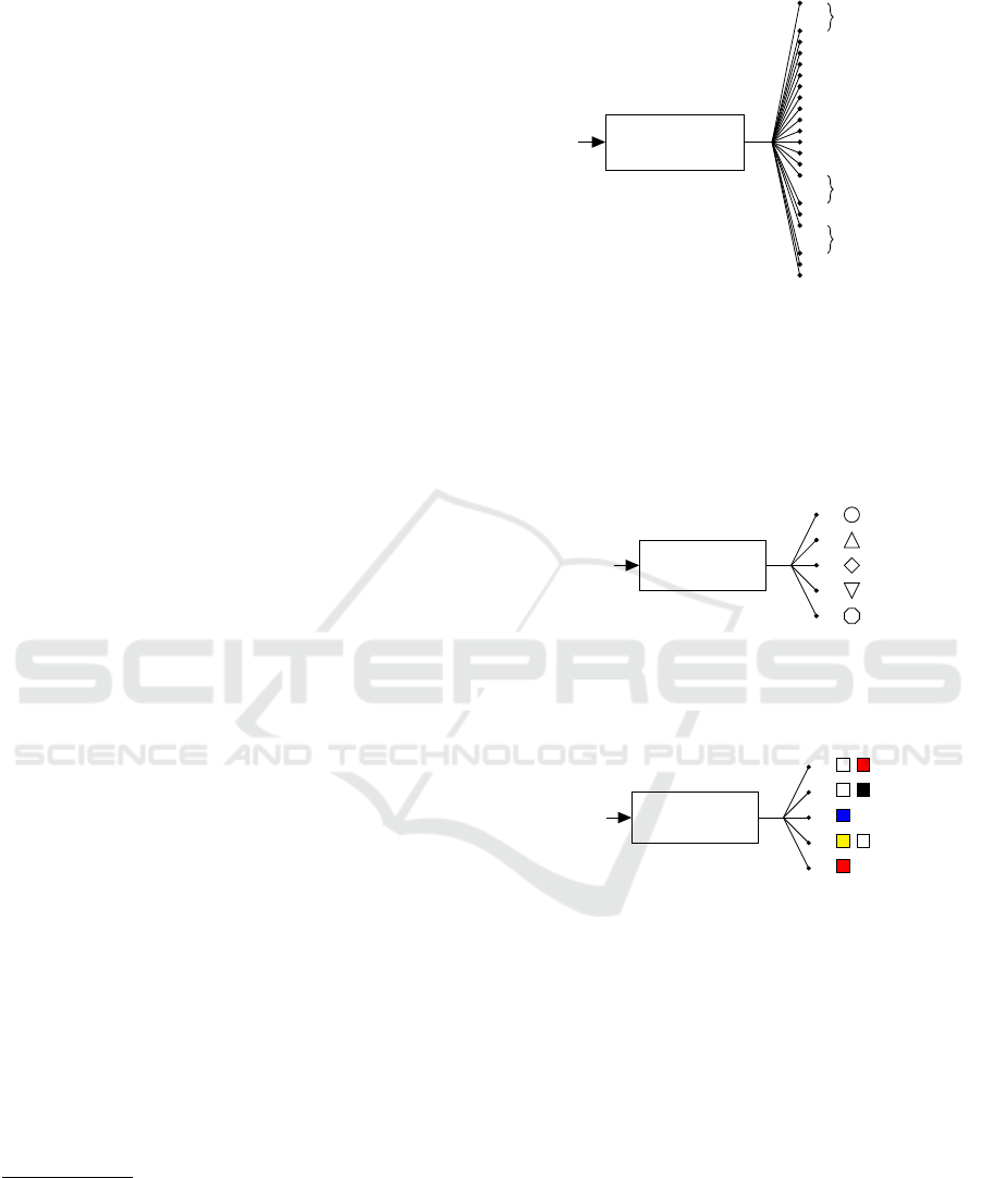
This is also shown in Figure 4.
4.2.2 Secondary Classifiers
Some traffic signs vary in terms of their physical char-
acteristics, i.e., variation in terms of shape, color or
both. However, all the traffic signs of a particular
sign type
7
have the same physical characteristics. The
classifier f
primary
, for a given input image, can experi-
ence either an inter-sign-type
8
misclassification or an
intra-sign-type
9
misclassification.
An inter-sign-type misclassification by f
primary
implies that it is perhaps not able to correctly visual-
ize the high-level feature(s) (i.e., shape and/or color)
of the traffic sign in the given input image. In or-
der to deal with such misclassifications, a suitable ap-
proach can be to implement two additional diverse
classifiers: one for predicting the shape of the traf-
fic sign and the other to classify the traffic sign based
on the prominent colors present on the sign board.
Since these classifiers focus on classifying the input
traffic sign image on the basis of just the correspond-
ing high-level feature, it is expected that these clas-
sifiers will be easier to train and have high accuracy.
We refer to these two secondary classifiers as shape
and color classifier, i.e., f
shape
and f
color
, respectively.
The classes to which these classifiers map the input
image X
X
X are presented in Figure 5. All the 43 traf-
fic signs in GTSRB can be grouped into the classes
{S
1
,S
2
,...,S
5
} and {C
1
,C
2
,...,C
5
} on the basis of the
shape of the traffic signs and the prominent colors
present on the sign boards, respectively. Mathemat-
ically, we represent the two classifiers as:
• Shape classifier f
shape
: X
X
X ∈ R
l
−→
ˆ
S
secondary
∈
{1,2,...,5}, and
7
the 39 traffic signs in GTSRB belong to one of the sign
types: speed limit, prohibitory, danger, mandatory and der-
estriction. The remaining 4 signs (priority road, yield to
cross, do not enter, stop) are independent sign types.
8
predicted traffic sign is of a type, different than that of the
actual traffic sign.
9
predicted traffic sign is of a type, same as that of the actual
traffic sign.
Primary Classifier
f
primary
Input
Image
X
X
X
1
.
.
6
SL (1-6)
7
DRT (1)
8
SL (7)
9
SL (8)
10
PROH (1)
11
PROH (2)
12
DNG (1)
13
Priority road sign
14
Yield to cross sign
15
Stop sign
16
PROH (3)
17
PROH (4)
18
Do not enter sign
19
.
.
32
DNG (2-15)
33
DRT (2)
34
.
.
41
MDT (1-8)
42
DRT (3)
43
DRT (4)
Predicted traffic sign (ˆy
primary
)
Figure 4: Primary classifier to predict the traffic sign class
in an input image X
X
X. The sign type for every traffic sign
class is also mentioned, where SL, DRT, PROH, DNG and
MDT denote the sign types: speed limit, derestriction, pro-
hibitory, danger and mandatory, respectively.
Shape Classifier
f
shape
Input
Image
X
X
X
Shape of the sign board
S
1
S
2
S
3
S
4
S
5
(a) Shape-type classifier
Color Classifier
f
color
Input
Image
X
X
X
Prominent colors on the sign board
(A = Background, B = Border)
A
B
C
1
C
2
C
3
C
4
C
5
(b) Color-type classifier
Figure 5: Shape and color type classifiers that are trained
for predicting the shape and the prominent colors on the
sign board in the input traffic sign image, respectively.
• Color classifier f
color
: X
X
X ∈ R
l
−→
ˆ
C
secondary
∈
{1,2,...,5}.
Let us consider that the classifiers f
shape
and f
color
predict
ˆ
S
secondary
= 2 (triangle pointed upwards) and
ˆ
C
secondary
= 1 (white background and red border) for
an input image X
X
X. This implies that they collaborate
to predict the sign type of the traffic sign in X
X
X as dan-
ger, since all the danger traffic signs are triangular
(pointed upwards) in shape and bear a white back-
ground with red border. Now, we use an additional
classifier f
dng
, which, unlike f
primary
, is trained to map
X
X
X into one of the 15 danger traffic sign classes only.
Similarly, we can train the additional classifiers for
the other sign types, namely, speed limit, prohibitory,
Deep Learning Classifiers for Automated Driving: Quantifying the Trained DNN Model’s Vulnerability to Misclassification
217

derestriction and mandatory. Note that all the speed
limit and the prohibitory traffic signs have the same
shape and bear the same prominent colors, therefore,
we train a common classifier f
sl/proh
with all the speed
limit and the prohibitory signs as the target classes.
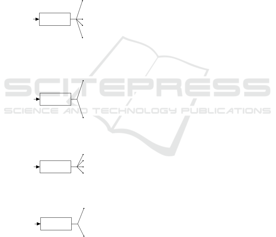
These sign type specific classifiers are schematically
represented in Figure 6, and their mathematical repre-
sentations are given below:
• Speed limit/prohibitory signs classifier f
sl/proh
:
X
X
X ∈ R
l
−→ ˆy
sl/proh
∈ {1,2, ...,12},
• Danger signs classifier f
dng
: X
X
X ∈ R
l
−→ ˆy
dng
∈
{1,2,...,15},
f
sl/proh
Input
Image
X
X
X
1
SL (1)
.
.
.
.
.
.
8
SL (8)
9
PROH (1)
.
.
12
PROH (4)
Predicted speed limit/
prohibitory sign (ˆy
sl/proh
)
(a) Speed limit/prohibitory signs classi-
fier
f
dng
Input
Image
X
X
X
1
DNG (1)
.
.
.
.
.
.
.
.
.
.
.
.
.
15
DNG (15)
Predicted danger sign
( ˆy
dng
)
(b) Danger signs classifier
f
drt
Input
Image
X
X
X
1
DRT (1)
2
DRT (2)
3
DRT (3)
4
DRT (4)
Predicted derestriction
sign ( ˆy
drt
)
(c) Derestriction signs classifier
f
mdt
Input
Image
X
X
X
1
MDT (1)
.
.
.
.
.
.
8
MDT (8)
Predicted mandatory
sign ( ˆy
mdt
)
(d) Mandatory signs classifier
Figure 6: Sign type specific classifiers, wherein all the cor-
responding target traffic sign classes have the same physical
characteristics (shape and prominent colors).
• Derestriction signs classifier f
drt
: X
X
X ∈ R
l
−→
ˆy
drt
∈ {1,2, ...,4}, and
• Mandatory signs classifier f
mdt
: X
X
X ∈ R
l
−→
ˆy
mdt
∈ {1,2, ...,8}.
Since the traffic signs: do not enter, priority road,
yield to cross and stop, are independent in terms of
their shape and color, we do not train any further sec-
ondary classifier(s). For instance, if f
shape
and f
color
predict
ˆ
S
secondary
= 5 (octagon) and
ˆ
C
secondary
= 5 (red
background) for an input image X
X
X, the prediction
obtained by the network of secondary classifiers is
stop sign. The traffic sign predicted upon the use
of the secondary classifiers is finally mapped back
into the corresponding original traffic sign label in
{1,2,...,43}, which is then considered as ˆy
secondary
.
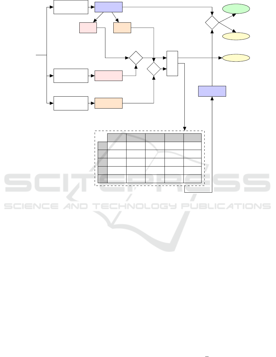
4.2.3 Merging the Decisions of the Classifiers
A schematic representation of the approach is pro-
vided in Figure 7. For a given input image X
X
X, if
the prediction made by the primary classifier f
primary
is 20 speed limit sign (i.e., ˆy
primary
= 1), then by
prior knowledge, we know that the shape of the
sign board will be circular (i.e.,
ˆ
S
primary
= S
1
) and it
will have a white background with red border (i.e.,
ˆ
C
primary
= C
1
). Now, the predictions
ˆ
S
secondary
and
ˆ
C
secondary
, made by the secondary classifiers f
shape
and
f
color
, are compared with
ˆ
S
primary
and
ˆ
C
primary
, respec-
tively. If either or both the conditions:
ˆ
S
primary
=
ˆ
S
secondary
and
ˆ
C
primary
=
ˆ
C
secondary
are false, then the fi-
nal prediction is an undecided outcome, i.e., ˆy
final
= φ.
On the contrary, if both the abovementioned condi-
tions are true simultaneously, then based on the pre-
dicted shape and color class (i.e.,
ˆ
S
primary
/
ˆ
S
secondary
and
ˆ
C
primary
/
ˆ
C
secondary
), the traffic sign prediction
ˆy
secondary
is derived from the matrix given in Figure
7. Again, the unanimity of the predictions ˆy
primary
and
ˆy
secondary
is checked. As also shown in Equation 17,
if both these predictions are the same, then the final
prediction ˆy
final
for the input image X
X
X is ˆy
primary
(or
ˆy
secondary
). However, non-unanimity results in an un-
decided outcome, i.e., ˆy
final
= φ.
The effectiveness of this mechanism is remarked
by it’s ability to trigger an undecided outcome for
all those test images for which the primary classifier
make incorrect predictions. Nevertheless, the disad-
vantage of this strategy is that it might also trigger an
undecided outcome for certain amount of test images
for which the primary classifier already make correct
predictions. Thus, a suitable threshold must be im-
posed to ensure that the number of test images for
which ˆy
final
= φ is not too high. However, defining
this threshold is not within the scope of this paper.
VEHITS 2021 - 7th International Conference on Vehicle Technology and Intelligent Transport Systems
218

Primary Classifier
f
primary
Predicted traffic sign
{1,2,..., 43}
ˆy
primary
ˆ
S
primary
Shape of the
predicted sign
{S
1
,S
2
,...,S
5
}
ˆ
C
primary
Prominent colors on
the predicted sign
{C
1
,C
2
,...,C
5
}
Shape Classifier
f
shape
ˆ
S
secondary
Predicted shape class
{S
1
,S
2
,...,S
5
}
Color Classifier
f
color
ˆ
C
secondary
Predicted color class
{C
1
,C
2
,...,C
5
}
Input
Image
X
X
X
equal ?
equal ?
AND
Undecided
FALSE
TRUE
Input:
Shape and
color class
ˆy
secondary
Predicted traffic sign
{1,2,..., 43}
equal ?
Final output
ˆy
primary
TRUE
Undecided
FALSE
Prediction of traffic signs
based on predicted shape
and color class
S
1
S
2
S
3
S
4
S
5
C
1
f
sl/proh
(X
X
X) f
dng
(X
X
X)
-
Yield to
cross sign
-
C
2
f
drt
(X
X
X)
- - - -
C
3
f
mdt
(X
X
X)
- - - -
C
4
- -
Priority road
sign
- -
C
5
Do not
enter sign
- - -
Stop sign
Figure 7: Prediction of the traffic sign class for the input image X
X
X by fusing the predictions of the primary classifier ( f
primary
)
and the network of secondary classifiers (i.e., f
shape
, f
color
, f
sl/proh
, f
dng
, f
drt
and f
mdt
).
4.3 Experimentation
A total of 26640 images from the GTSRB training
data were splitted into three equal subsets. All the im-
ages were rescaled to l = 48×48×3 pixels. The first
subset of the data was used to train the primary clas-
sifier f
primary
. The model f used for our analysis in
Section 3.4 is f
primary
in our experimentation here.
Half of the images in the second subset of the
training data were used to train the shape classifier
f
shape
, while the other half were used to train the color
classifier f
color
. For training the classifiers f
shape
and
f
color
, the images in their respective training data were
first mapped from the traffic sign classes {1, 2, ...., 43}
into the corresponding shape {S
1
,S
2
,S
3
,S
4
,S
5
} and
color {C
1
,C
2
,C
3
,C
4
,C
5
} classes, respectively. The
shape and the color classes (shown in Figure 5) were,
hence, used as labels for training f
shape
and f
color
, re-
spectively. The images in the third subset belonging
to the speed limit and prohibitory sign types were
used to train the classifier f
sl/proh
, and similarly, the
other classifiers, i.e., f
dng
, f
drt
and f
mdt
were trained
with the corresponding sign type’s images in the third
subset of the training data. Further experimenta-
tion details (e.g., DNN architecture, hyperparameters,
etc.) related to the training and the evaluation of these
classifier models are recorded in Appendix B. Note
that the set of test images, i.e., X
test
, used for the eval-
uation here is the same as used in Section 3.4.3.
4.4 Results and Discussion
4.4.1 Evaluation of the Mechanism
Firstly, the individual accuracies of the classifier mod-
els are recorded in Table 1.
Let us denote the total number of test images used
for the evaluation as τ. When we use the primary clas-
sifier alone (i.e., without the implementation of the
mechanism), let us assume it misclassifies ρ number
of images. The misclassification rate by f
primary
is:
¯
ρ =
ρ
τ
× 100. (18)
Now, when we implement the mechanism, out of
these τ test images, let us say that the mechanism
Deep Learning Classifiers for Automated Driving: Quantifying the Trained DNN Model’s Vulnerability to Misclassification
219

Table 1: Individual accuracies of the classifier models.
Classifier # Test Images Test Accuracy
f
primary
10000 96.12 %
f
shape
10000 98.87 %
f
color
10000 98.56 %
f
sl/proh
4497 98.2 %
f
dng
2207 95.7 %
f
drt
278 94.6 %
f
mdt
1409 97.3 %
yields an undecided outcome (i.e., ˆy
final
= φ) for λ im-
ages. Thus, the percentage of test images for which
the mechanism does not yield any prediction is:
¯u =
λ
τ
× 100. (19)
The number of images for which ˆy
final
= ˆy
primary
is (τ − λ). Let us assume that out of these (τ − λ)
images, for ω images the final prediction (i.e., ˆy
final
=
ˆy
primary
) is actually an incorrect prediction. Therefore,
the misclassification rate after the implementation of
the mechanism becomes:
¯
ω =
ω
τ − λ
× 100. (20)
We use the mechanism presented in Figure 7 to
obtain the final prediction ( ˆy
final
), for all the τ =
10000 images in the set of original GTSRB test data,
i.e., X
test
, as well as for the set of perturbed test im-
ages, i.e., X
∆contrast
, X
∆brightness
, X
∆blur
and X
∆noise
.
The obtained values of
¯
ρ (Equation 18), ¯u (Equa-
tion 19) and
¯
ω (Equation 20) are determined for each
of these sets of test images. The results are pre-
sented in Figure 8. To realize the advantage of us-
ing the mechanism, we compare the misclassification
rate
¯
ω obtained after implementation of the mecha-
nism with the misclassification rate
¯
ρ observed when
using f
primary
alone. In Figure 8, consider the results
corresponding to X
test
. The use of f
primary
alone re-
sults in a misclassification rate of
¯
ρ = 3.88%. How-
ever, when the mechanism is used, for ¯u = 5.61% of
images in X
test
, no decision is produced. Among the
remaining images, i.e., for which a decision is pro-
duced ( ˆy
final
= ˆy
primary
), the misclassification rate is
just
¯
ω = 0.69%. A substantial drop in the misclas-
sification rate suggests that the mechanism controls
the misclassifications incurred by f
primary
consider-
ably well. Similar conclusion can be drawn from the
results obtained for the set of perturbed test images.
4.4.2 Validation of the Arguments 1 and 2
For the test data X
test
, X
∆contrast
, X
∆brightness
, X
∆blur
and X
∆noise
, the number of images n
low
, n
moderate
, and
n
high
misclassified by f
primary
are already shown in
Figure 3. For instance, consider the set of the original
(unperturbed) test images, i.e., X
test
. The values are
n
low
= 1, n
moderate
= 103, and n
high
= 284 (Figure 3a).
As discussed in Section 4.1, we expect the mechanism
in Figure 7 to yield ˆy
final
= φ (undecided outcome),
ideally, for all these images misclassified by f
primary
.
Upon investigation, we observed that the mechanism
does yield the undecided outcome for the n
low
= 1 im-
age, and hence, ¯u
low
= 100%. The term ¯u
low
signifies
the percentage of n
low
images for which the mecha-
nism does not yield any decision. Out of n
moderate
=
103 images, the mechanism yields the undecided out-
come for 97 images, i.e., 94.17% of n
moderate
im-
ages. Therefore, ¯u
moderate
= 94.17%. However, out
of n
high
= 284 images, the mechanism yields the un-
decided outcome for only 225 images, i.e., 79.23% of
n
high
images, therefore, ¯u
high
= 79.23%. We continue
this investigation for the set of perturbed test images.
The results are presented in Table 2. It is observed
that for all the n
low
number of misclassified images
(i.e., for which the corresponding misclassifications
lie in M
low
), the mechanism yields the undecided out-
0
2
4
6
8
10
12
14
Figure 8: Experimental results: Evaluation of the mechanism.
.
VEHITS 2021 - 7th International Conference on Vehicle Technology and Intelligent Transport Systems
220

Table 2: Experimental results: Validation of the arguments.
Test Images
For the misclassification(s) belonging to:
M
low
M
moderate
M
high
n
low
¯u
low
n
moderate
¯u
moderate
n
high
¯u
high
Original X
test
1 100% 103 94.17% 284 79.23%
Perturbed
Contrast change X
∆contrast
4 100% 112 95.54% 299 85.62%
Brightness change X
∆brightness
15 100% 156 91.03% 533 81.05%
Gaussian blur X
∆blur
2 100% 138 89.13% 425 79.53%
Gaussian noise X
∆noise
27 100% 197 88.32% 564 69.33%
come. On the other hand, it is relatively difficult to
achieve the same for all the n
high
number of misclas-
sified images (i.e., for which the corresponding mis-
classifications lie in M
high
). It can be inferred that the
misclassifications that were ranked to be offering the
primary classifier model a high vulnerability (based
on our categorisation criteria) are relatively difficult
to control, even after the implementation of the ad-
ditional efforts to minimize the misclassification rate.
One can expect the amount of rigor required to control
a particular misclassification incurred by f
primary
to be
considerably higher as it’s vulnerability to the mis-
classification increases. The investigation supports
our Arguments 1 and 2 specified in Section 4.1.
5 CONCLUSIONS
In this paper, we proposed an approach to estimate
how vulnerable is a trained DNN model to any par-
ticular misclassification. It is based on estimating
the DNN’s vulnerability to misclassification of an in-
put image belonging to a class k
1
into an incorrect
class k
2
by measuring the similarity learnt by the
trained model between the classes k
1
and k
2
. We il-
lustrated experimentally that the majority of the test
images that are misclassified by the model encounter
the misclassifications to which it’s vulnerability is cat-
egorised as high. This provides a rationale to our
proposed approach and also justifies its potentiality
to identify the set of critical misclassifications that
the DNN model is more likely to incur during the
operation. Based on the acquired knowledge, perti-
nent measures or counter strategies can be developed
and integrated to curb the in-operation likelihood of
these critical misclassifications. Our further empir-
ical investigation was to validate the argument that
the amount of rigor required to deal with these crit-
ical misclassifications is relatively higher than what is
required to deal with the misclassifications to which
the DNN model is moderately or lowly vulnerable.
As an extension to this work, we wish to study how
the knowledge acquired by the application of this pro-
posed concept be further utilized for the preparation
of the consequent steps to enhance the robustness
and/or performance of the image classification func-
tionality in highly automated driving.
ACKNOWLEDGEMENTS
We thank the anonymous reviewers for their valuable
comments and feedback.
REFERENCES
Agarwal, H., Dorociak, R., and Rettberg, A. (2020). A
strategy for developing a pair of diverse deep learn-
ing classifiers for use in a 2-classifier system. In 2020
X Brazilian Symposium on Computing Systems Engi-
neering (SBESC), pages 1–8. IEEE.
Agarwal, H., Dorociak, R., and Rettberg, A. (2021). On
developing a safety assurance for deep learning based
image classification in highly automated driving. In
2021 Design, Automation & Test in Europe Confer-
ence (DATE).
Chollet, F. et al. (2015). Keras. https://keras.io.
Gao, X. W., Podladchikova, L., Shaposhnikov, D., Hong,
K., and Shevtsova, N. (2006). Recognition of traf-
fic signs based on their colour and shape features
extracted using human vision models. Journal of
Visual Communication and Image Representation,
17(4):675–685.
Grigorescu, S. M., Trasnea, B., Cocias, T., and Mace-
sanu, G. (2019). A survey of deep learning tech-
niques for autonomous driving. arXiv preprint
arXiv:1910.07738.
Harris, C. R. et al. (2020). Array programming with
NumPy. Nature, 585:357–362.
Hunter, J. D. (2007). Matplotlib: A 2d graphics environ-
ment. Computing in Science & Engineering, 9(3):90–
95.
Kashyap, R. (2019). The perfect marriage and much more:
Combining dimension reduction, distance measures
and covariance. Physica A: Statistical Mechanics and
its Applications, 536:120938.
Krizhevsky, A., Sutskever, I., and Hinton, G. E. (2012).
Imagenet classification with deep convolutional neu-
ral networks. In Pereira, F., Burges, C. J. C., Bottou,
Deep Learning Classifiers for Automated Driving: Quantifying the Trained DNN Model’s Vulnerability to Misclassification
221

L., and Weinberger, K. Q., editors, Advances in Neu-
ral Information Processing Systems, volume 25, pages
1097–1105. Curran Associates, Inc.
Muhammad, K., Ullah, A., Lloret, J., Del Ser, J., and de Al-
buquerque, V. H. C. (2020). Deep learning for safe
autonomous driving: Current challenges and future
directions. IEEE Transactions on Intelligent Trans-
portation Systems.
Ouyang, W., Zhou, H., Li, H., Li, Q., Yan, J., and Wang,
X. (2017). Jointly learning deep features, deformable
parts, occlusion and classification for pedestrian de-
tection. IEEE transactions on pattern analysis and
machine intelligence, 40(8):1874–1887.
Pedregosa, F. et al. (2011). Scikit-learn: Machine learning
in Python. Journal of Machine Learning Research,
12:2825–2830.
Ribeiro, M. T., Singh, S., and Guestrin, C. (2016). ”Why
Should I Trust You?”: Explaining the Predictions of
Any Classifier. arXiv preprint arXiv:1602.04938.
SAE International (2014). Taxonomy and Definitions for
Terms Related to On-Road Motor Vehicle Automated
Driving Systems (Standard No. J3016).
Sermanet, P., Eigen, D., Zhang, X., Mathieu, M., Fergus,
R., and LeCun, Y. (2014). Overfeat integrated recog-
nition, localization and detection using convolutional
networks. In 2nd International Conference on Learn-
ing Representations, ICLR 2014.
Stallkamp, J., Schlipsing, M., Salmen, J., and Igel, C.
(2012). Man vs. computer: Benchmarking machine
learning algorithms for traffic sign recognition. Neu-
ral Networks, 32:323–332.
Tian, Y., Zhong, Z., Ordonez, V., Kaiser, G., and Ray, B.
(2020). Testing DNN image classifiers for confu-
sion & bias errors. In Proceedings of the ACM/IEEE
42nd International Conference on Software Engineer-
ing, pages 1122–1134.
Virtanen, P. et al. (2020). SciPy 1.0: Fundamental Algo-
rithms for Scientific Computing in Python. Nature
Methods, 17:261–272.
Zhu, Y., Zhang, C., Zhou, D., Wang, X., Bai, X., and
Liu, W. (2016). Traffic sign detection and recognition
using fully convolutional network guided proposals.
Neurocomputing, 214:758–766.
APPENDIX
A Primary Classifier
All the images from the GTSRB dataset were rescaled
to 48 × 48 × 3 and normalized so as to keep the pixel
values in the range of 0 to 1. For the experimenta-
tion details corresponding to the DNN model f (or
f
primary
), refer to the first row of Table 3.
B Secondary Classifiers
Table 3 also summarizes the details corresponding to
f
shape
, f
color
, f
sl/proh
, f
drt
, f
dng
and f
mdt
. From the val-
idation (and the test) data used for evaluating f
primary
,
f
shape
and f
color
, only the images belonging to the
sign type: speed limit/prohibitory, derestriction, dan-
ger and mandatory were used as the validation (and
the test) data for the corresponding sign type classi-
fiers, i.e., f
sl/proh
, f
dng
, f
drt
and f
mdt
, respectively.
Table 3: Experimentation details corresponding to the different classifier models.
Classifier
a
Brief Summary of the DNN
Architecture
b
Hyperparameters
c
Number of Images
Train Validation Test
f or
6 convolutional, 4 max pooling, 2
dense and 7 dropout layers
bs=64, α=10
−4
,
ϕ=10
−4
8880 2630 10000
f
primary
f
shape
3 convolutional, 3 max pooling, 2
dense and 4 dropout layers
bs=32, α=10
−4
,
ϕ=10
−4
4440 2630 10000
f
color
3 convolutional, 3 max pooling, 2
dense and 4 dropout layers
bs=32, α=10
−4
,
ϕ=10
−4
4440 2630 10000
f
sl/proh
8 convolutional, 4 max pooling, 4
dense and 8 dropout layers
bs=16, α=10
−4
,
ϕ=10
−4
3890 1173 4497
f
dng
8 convolutional, 4 max pooling, 4
dense and 12 dropout layers
bs=16, α=10
−3
,
ϕ=10
−4
2050 583 2207
f
drt
8 convolutional, 4 max pooling, 4
dense and 8 dropout layers
bs=16, α=10
−3
,
ϕ=10
−4
280 82 278
f
mdt
8 convolutional, 4 max pooling, 4
dense and 8 dropout layers
bs=16, α=10
−4
,
ϕ=10
−4
1280 361 1409
a
Every classifier was trained for 30 epochs using the standard categorical cross entropy loss function. We chose the model
obtained from the training epoch at which the highest validation accuracy was observed.
b
The DNN architecture yields two outputs: logits and output from the final softmax activation layer.
c
bs, α and ϕ denotes the batch size, the learning rate, and the learning rate decay, respectively.
VEHITS 2021 - 7th International Conference on Vehicle Technology and Intelligent Transport Systems
222