
Energy Optimal Control of a Multivalent Building Energy System
using Machine Learning
Chenzi Huang, Stephan Seidel, Xuehua Jia, Fabian Paschke and Jan Bräunig
Fraunhofer Institute of Integrated Circuits IIS, Division Engineering of Adaptive Systems EAS,
Zeunerstraße 38, 01069 Dresden, Germany
Keywords: Reinforcement Learning, Model Predictive Control, Building Energy System, Machine Learning.
Abstract: In this contribution we develop and analyse intelligent control methods in order to optimise the energy
efficiency of a modern residential building with multiple renewable energy sources. Because of alternative
energy production options a non-convex mixed-integer optimisation problem arises. For the solution we first
apply combined optimisation methods and integrate it into a model predictive controller (MPC). In
comparison, a reinforcement learning (RL) based approach is developed and evaluated in detail. Both
methods, in particular reinforcement learning approaches are able to decrease energy consumption and keep
thermal comfort at the same time. However, in this paper RL can achieve better results with less computational
resources than MPC approach.
1 INTRODUCTION
Since buildings still account for about of
Germany's primary energy consumption, the field of
building automation and energy management has
increasingly become a focus of current research
(BMWi, 2019). In addition to structural methods,
such as improving building insulation, there is also a
high saving potential that can be achieved by the
building automation system itself. Considering the
increasing use of varying renewable energy sources
and storage systems, new methods such as model
predictive control and machine learning based control
approaches receive more and more attention (Renaldi,
2017 and Oldewurtel 2012). Especially algorithms
from the field of reinforcement learning are
particularly attractive (Chen, 2018 and Mason, 2019),
since they pursue the goal of independent learning
strategies in order to maximise a certain profit,
whereby the short-term profit can be weighed against
the accumulating long-term profit.
The central energy control system, also referred to
as energy manager (EM), usually cannot access local
controllers, such as control parameters of dedicated
room controllers, in practice. Instead the EM should
take higher-level, possibly binary, decisions. This
includes the temporal on-off behaviour of certain
energy consumers (demand-side management
(Palensky and Dietrich, 2011)) or generators and
distributors (e. g. pumps or heatpumps).
Mathematically, this results in (mixed-) integer
optimisation problems with a large number of
decision variables, that often can not be solved in
reasonable time. Thus, intelligent mathematical
approaches are needed, that are also applicable to a
large number of energy producers and consumers in
practice. In the last years the authors have analysed
and developed several approaches in order to design
and implement energy saving control algorithms for
both heat/energy consumption and generation system.
These used methods include simulation-based design
and optimisation (Seidel, 2015), model-predictive
control (Paschke, 2016) as well as data analysis
(Paschke, 2020) for predictive maintenance and
condition monitoring.
In this contribution we focus on the design of an
energy management system for a modern residential
building, with multiple renewable sources and storage
systems. Thus, we will first introduce a model of the
energy system of the building. In the subsequent
section, for the design of the energy manager the
decision variables and the constraints of the
optimisation problem will be stated. Section 4 and 5
describe the implementation details of a model
predictive control and a reinforcement learning based
control methods, respectively. Finally, both
approaches will be compared in Section 6 and a
summary and an outline of future work will be
Huang, C., Seidel, S., Jia, X., Paschke, F. and Bräunig, J.
Energy Optimal Control of a Multivalent Building Energy System using Machine Learning.
DOI: 10.5220/0010478500570066
In Proceedings of the 10th International Conference on Smart Cities and Green ICT Systems (SMARTGREENS 2021), pages 57-66
ISBN: 978-989-758-512-8
Copyright
c
2021 by SCITEPRESS – Science and Technology Publications, Lda. All rights reserved
57
presented.
2 MODELING OF THE
BUILDING ENERGY SYSTEM
The model of the building energy system is used as
the process model of the designed energy manager. It
is based on a 2007-built residential building, but was
simplified in order to reduce runtime for simulation
and optimisation. The real-world building is a
detached house with 2 floors and around 300m² living
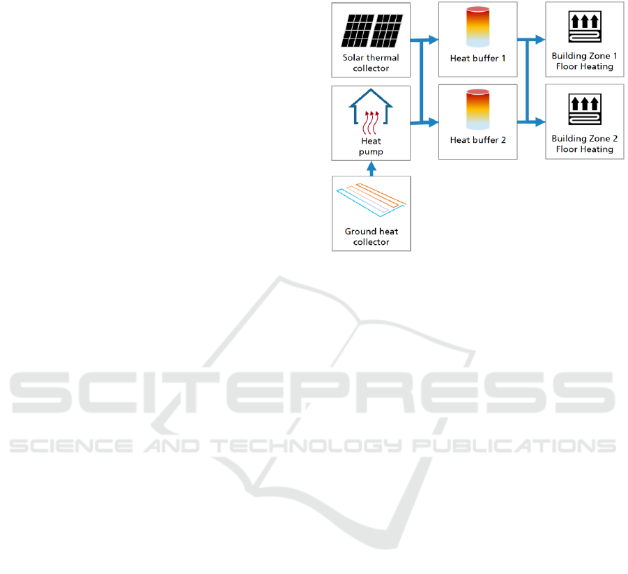
space. It is composed of the following subsystems
(see Fig. 1) for heat generation, buffering and
consumption:
Solar Thermal System. A solar thermal system
(STS) is installed on the roof of the building that can
heat up the water in one of the two buffer tanks. The
STS has a simple local control system that enables the
pump of the collector if an adjustable temperature
difference between the collector and the buffer tank
is exceeded. The volume flow is controlled depending
on the difference between the flow and return
temperature. The STS can be activated and
deactivated by the EM.
Geothermal System. The base load of the heat
supply is provided by a brine-water heat pump (HP)
with a ground heat collector. The environmental heat
extracted by the heat pump is buffered also in these
two heat storage tanks. The temperature in the storage
tanks is controlled by bang-bang control, thus the heat
pump is switched on if the temperature in one of the
tanks falls below its desired value. The tanks are filled
alternately.
Thermal Storages. As mentioned previously, the
energy system of the building has two buffer tanks.
The tanks provide heat for the building and have a
volume of 1250l each. Because of the small size a
frequent recharge is necessary, especially in winter.
Building and Automation System. The building
model consists of one storey with two
thermal zones that are oriented north and south,
respectively. Occupancy and internal loads have been
neglected. The zones are heated by a floor heating
system that is controlled by two autonomous
controllers. The temperature setpoints of 21 and 23°C
are lowered by 1K depending on the daytime and
weekday.
2.1 Environment
Weather data, such as outside temperature and solar
radiation, from a test reference year (TRY) of
Dresden has been used as input to the model.
Figure 1: Structure of the building heating/energy
system.
2.2 Simulation
The model of the building and the energy system was
implemented and simulated with SimulationX of ESI.
The energy system was modelled with the GreenCity-
Library, whereas the local controllers of the STS and
HP where implemented with the Modelica Standard
Library (MSL). The energy system was modelled
such that no EM is necessary, meaning that the task
of providing heating energy to the building can be
accomplished by the local controllers as well. This
scenario corresponds to a standard approach, where
the heat demand is covered by the STS and HP
together, which can be inefficient if for example the
HP is switched on although the STS can provide
enough heat. This inefficiencies are addressed by the
subsequently described optimisation approaches that
are validated using the described model.
2.3 Implementation of MPC and RL
The development of complex control algorithms,
such as MPC and RL, is not possible within
SimulationX. Hence, an export of the whole model is
necessary so that it can be accessed by external
software. Thus, using the FMI Standard (Blochwitz,
2011), the model was exported into a Functional
Mock-Up Unit (FMU). The implementation of the
MPC and RL-based control algorithms was then done
using Python and FMPy (Dassault Systems, 2017),
that provides an interface for the import and
execution of the FMU.
SMARTGREENS 2021 - 10th International Conference on Smart Cities and Green ICT Systems
58

3 ENERGY MANAGER
According to the model of the building energy
system, the high level building energy manager which
we design is going to make three decisions: 1.
Selection of the appropriate heat source for energy
production; 2. Selection of the thermal storage to save
the produced energy; 3. Selection of the thermal
storage for heating. More precisely, the following
discrete control inputs need to be determined:
-
: Enable-signal for heat pump to use the
geothermal system
-
: Enable-signal for solar heat
-
: Load thermal storage 1 or 2 with
heat from heat pump
-
: Load thermal storage 1 or 2 with
solar heat
-
: Signals to discharge thermal storage 1 or
2 for heating.
This leads to the control input vector
For a given time horizon , the energy manager
has to propose a control input function
or
if is
divided into discrete time samples.
Since each of the 8 control inputs are Boolean, for
time samples, there are
possible solutions for
. In addition, there are some constraints to be
considered. They are based on the real system
configuration and are listed in Table 1.
Table 1: Constraints.
Only one storage shall be used for
heating.
Solar heat can be used to load both
thermal storages
Thermal storage 1 shall not be
charged via heat pump.
* For particularly cold days, both
storages can be charged via heat
pump and both can be used for
heating at the same time.
3.1 Optimisation Problem
For a concrete cost function , we can note the
following general discrete optimisation problem:
(1)
Here describes the model of the building energy
system, and represent the constraints to be
considered where according to Table 1 their concrete
functions only depend on , not on .
For the cost function two main factors are taken
into account:
1. Comfort violation.
In this paper comfort violation is indicated by the
deviation of the room temperature from the set
temperature
. The set temperature values depend
on the hour of the day and the weekday. A simple
choice for cost calculation is:
(2)
where
is the temperature of the i-th thermal zone.
Considering the concept of thermal comfort (Gao,
Li and Wen, 2019), which subjectively reflects the
satisfaction of people under certain thermal
conditions, such as too cold, cold, neutral, warm and
too warm, the extent of temperature deviation
can
also be punished differently as follows:
(3)
In particular, we do not punish the case where the
temperature is above the set temperature, since the
building energy system does not have active cooling.
For both kind of cost definition, if temperature is
given as vectors
and
of length , the comfort
cost can then be calculated as the sum of all
-
elements:
(4)
or be calculated from the average value
of the
vector
:
(5)
Energy Optimal Control of a Multivalent Building Energy System using Machine Learning
59

2. Electrical energy
.
Here we consider the electrical power consumed by
the pumps (e.g. heat pump and pump of solar thermal
system) for heating. This contradicts the first target of
minimizing comfort violation. So for optimisation a
trade-off of both targets is pursued.
Therewith, we have
(6)
where
and
and
are the weighting factors.
Since the general optimisation problem
formulated in eq. (1) is discrete with integer
optimisation variables, we have a so-called
constrained integer nonlinear problem, which belongs
to the class of mixed integer nonlinear problem
(MINLP).
3.2 Solution Approach
For a general MINLP there are different state-of- the-
art solution approaches, e.g. the use of regularisation
techniques where the exact knowledge of model
equations is required (Mynttinen, 2015), optimisation
methods combining constraint programming and
nonlinear optimisation programs especially for
scheduling problems (Wigström and Lennartson,
2012 and 2014), and complex heuristic optimisation
methods (Schlüter et Al, 2009).
In this paper, based on the concept from
(Wigström and Lennartson, 2014), we designed a
solution approach which at first simplifies problem
(1) using constraint programming technique, such
that at the second step, a less complex optimisation
strategy can be applied.
Constraint programming (CP) is generally used to
find solutions of a problem with declarative stated
constraints. It can be applied in our case as a first step
to find those solutions of satisfying the
nonlinear constraint equations. Here we take
advantage of the fact that the constraint functions
and according to Table 1 do not depend on internal
states of the building. With an appropriate CP-
solver, the solution space of problem (1) can be
reduced:
. Without regard to last
constraint (*) only 16 feasible solutions instead of
remain. The case (*) can be taken into account
if the charge of both storages via heat pump and the
simultaneous discharge of both is allowed. This
additional solution can be added to
.
As a result, problem (1) can be simplified to an
integer optimisation problem without constraints:
(7)
where
summarizes and the building model . This
remaining problem needs to be linked with an
appropriate solver and integrated into the energy
manager for the control of the active building heating
system.
In this paper we investigate two control strategies.
The first is to integrate the optimisation problem
stated above into a classic model predictive control
where problem (7) can be solved by an appropriate
heuristic optimisation method. The second is to use
machine learning approaches, in particular, we have
our focus on reinforcement learning. Both approaches
are presented in the following sections.
To evaluate the benefits of these approaches, we
compare their results with the behaviour of the basic
building automation system where constraints from
Table 1 are neglected. In that case the heat pump is
activated according to the temperature level of each
of the storages (here storage 1 can always be loaded
via heat pump) and both storages are simultaneously
and equally used for heating. This basic building
control configuration will be subsequently denoted as
NC (for no high level control).
4 MODEL PREDICTIVE
CONTROL
4.1 Implementation
In case of MPC the optimisation problem (7) needs to
be solved repeatedly at each time step for upcoming
time horizon. In this paper, a simple form of genetic
algorithm (GA) is applied as the optimisation solver.
In order to determine appropriate optimisation
parameters, e.g. population size, number of
generations and weighting factors, a parameter
variation study has been conducted.
The model predictive control is implemented in
Python where the building model is integrated as
FMU. For first analysis the FMU serves not only as
the prediction model within MPC, but also as
simulation model for obtaining building state. The
time horizon is set to 24h and the time step is set to
3h in order to reduce the optimisation effort. This is
acceptable insofar that the energy system is
sufficiently slow. However, for dealing with fast
changing environmental changes, the time step needs
to be reduced in future.
Moreover, we compare the results using different
comfort calculations given by eq. (2) denoted as R1
and eq. (3) denoted as R2, using eq. (4).
SMARTGREENS 2021 - 10th International Conference on Smart Cities and Green ICT Systems
60
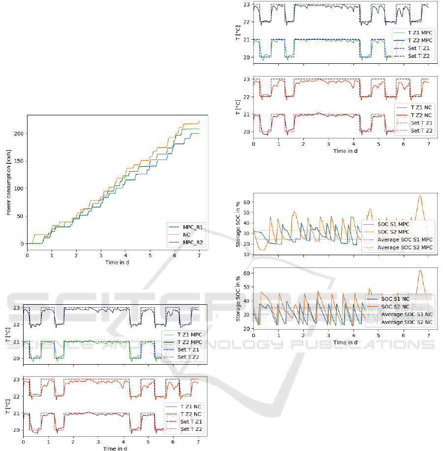
4.2 Simulation Result
In Fig. 2 – 4 the power consumption and the tempe-
rature of both thermal zones for 7 days in februrary
(starts from Thursday) are presented for MPC and NC.
Both versions of MPC with different comfort cost
calculation can reduce the power consumption of the
energy system of around for R1 and for
R2. Also the comfort level can be improved.
Figure 2: Comparison of total electric power consumption
between NC, MPC_R1 and MPC_R2.
Figure 3: Temperature in zone1 (Z1) and zone 2 (Z2). top:
MPC_R1, below: NC.
The energy saving is due to less charging of both
thermal storages by heat pump while still covering the
energy demand of both thermal zones. In particular,
the average soc of both storages has been reduced
compared to soc-level from NC. In case of R2, the soc
for storage 1 and 2 are 19% and 6% less compared to
NC (see Fig. 5).
Figure 4: Temperature in zone1 (Z1) and zone 2 (Z2). top:
MPC_R2, below: NC.
Figure 5: State of charge in
and
, top: MPC, below:
NC.
This result is of course based on the ideal setting that
the prediction model is exact. Moreover, eventhough
the potential of such a high level energy manager with
MPC is obvious, the computational effort and
hardware demand of online optimisation cannot be
neglected, especially when dealing with more
complex energy systems. Therfore, in the next section,
we will analyse and evaluate the application of
reinforcement learning where such an online
optimisation is not needed.
5 MACHINE LEARNING
APPROACHES
As a subset of artificial intelligence (AI) machine
learning (ML) is concerned with how to construct
computer programs that automatically improved with
experience (Jordan and Mitchell, 2015). Unlike the
conventional rule-based programming these
Energy Optimal Control of a Multivalent Building Energy System using Machine Learning
61

approaches use sufficient data and algorithms to
“train” the machine and make it capable to complete
tasks by themselves.
5.1 Reinforcement Learning
Reinforcement learning (RL) is a form of ML, which
is appropriate in solving complex optimal control
problems above through the interaction between
controller (AI agent) and system (environment). The
agent learns by trial and error and is rewarded for
taking desirable actions in a dynamic environment so
as to maximize cumulative rewards (Sutton and
Barton, 2018). Among all the perspectives on RL
algorithms we focus on the commonly used model-
free algorithms Q-learning and SARSA.
5.1.1 Markov Decision Process
We formulate the thermal comfort control and energy
optimisation of the building as Markov Decision
Process (MDP), which consists of a set of states and
actions , transition probability function , reward
function and the discount factor γ. Since the
interaction involves a sequence of actions and
observed rewards in discrete time steps
(the sequence is fully described by one
episode), the agent observes at each step the current
state (
) of the environment and decides on an
action (
) to take next according to a selection
policy
. Which state the agent will arrive in
is decided by
. Once an action is taken,
the environment delivers an immediate reward
as feedback. These steps will be iterated
during the learning phase and the control policy will
be updated until it is converged. Our purpose is to find
the maximum of the future reward over the episode,
which can be typically represented by the optimal Q
value (Szepesvári, 2010).
State. The relevant state of the MDP in this case is
occupation of the room, state of charge of the thermal
storage tank
and
and ambient temperature
at each time slot, represented as:
(8)
Action. The action of the MDP is equivalent to the
inputs signals of the system in section 3.
Reward. The reward of the MDP can be calculated
as the opposite of the cost function in section 3:
(9)
In the following, the reward function resulted from
comfort cost definition (eq. (3)) will be noted as
,
and from temperature difference definition (eq. (2))
as
, with eq. (5) for vectors.
Value Function. The estimated future reward in a
given state, also known as return, is a total sum of
discounted rewards going forward, mathematically
represented as follow:
(10)
The discount factor
penalizes the rewards
in the future, that may have a higher uncertainty and
does not provide immediate benefits.
The expected return can be represented as an
state-action value function/Q-function:
,
(11)
which can be decomposed into the immediate reward
plus the discounted future values by Bellmen
equations, and further by following the policy :
(12)
Temporal-Difference Learning. Since the agent
doesn’t know the state transition function before
the learning phase, we can’t solve the MDP directly
applying Bellmen equations, but using temporal
difference (TD) learning, which provides the agent
with a method to learn the optimal policy implicitly.
The value function Q will be updated towards the
estimated return
mathematically represented as follow:
(13)
where
is the learning rate, which controls
the extent of the update.
Selection Policy. The state transition in this case is
stochastic and the optimal policy in current state
will select whichever action maximizes the expected
return from starting in . As a result, if we have the
optimal value
, we can directly obtain the optimal
action
:
(14)
It’s common to balance the frequency of
exploring and exploiting actions with the ε-greedy
strategy, which chooses a randomly selected action
with probability
and otherwise according
to eq. (14).
SMARTGREENS 2021 - 10th International Conference on Smart Cities and Green ICT Systems
62
5.1.2 Control Strategy
SARSA (eq. (15)) and Q-learning (eq. (16)) are two
of the classic algorithms using TD learning (eq. (13)).
(15)
(16)
The key difference between SARSA and Q-
learning is that Q-learning is an off-policy but
SARSA an on-policy. It means that the Q-learning
agent doesn’t follow the current policy to pick the
next action. It estimates the optimal
, but the action
which leads to this maximal value may not be
followed in the next step.
5.2 Implementation
The proposed RL algorithms were implemented in
Python. The complete multivalent building energy
system was integrated as FMU.
At the beginning of each episode, the FMU model
will be instantiated anew and the initial states and as
well as all variables and parameters required by the
RL agent from the building environment will be
obtained. The state-action space is represented as a
matrix, i.e. Q table, which starts with a zero
matrix. During the training procedure the RL agent
can improve the control strategy based on the update
of the Q value in this table.
5.3 Simulation Result
5.3.1 Experimental Setup
In order to make all possible situations during the
training occur, in other words, to fill the blank initial
Q table, we train the model for a period of the whole
year (from 1st January until 31th December), and the
training episodes are set to 100. The first 7 days in
February are used to test the performance of the
energy management. The simulation step size for the
model internal is set to 5 minutes and the duration of
each time slot for the RL algorithm within one
training episode is 30 minutes. Additionally, the
hyperparameters settings such as learning rate α,
discount factor γ, exploration rate ε and the weighting
factors are varied between Q-learning and SARSA.
The adjustment of these hyperparameters is
performed manually and the final selection is listed in
Tab.2.
Table 2: Selection of the hyperparameters.
ε
γ
ε
Q-learning
0.95
0.9
0.6
1
150
150
1
20
25
SARSA
0.5
0.8
0.6
1
150
150
Besides that, the performance of our RL
algorithms is compared respectively with a default
scenario using static control/baseline approach,
precisely, a dummy agent with fixed action/control
inputs that are all set to true.
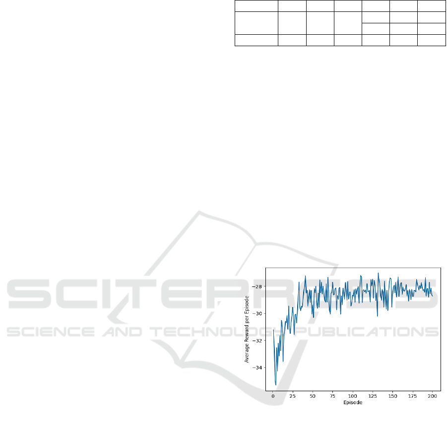
5.3.2 Performance Comparison
As mentioned before, the main objective of RL agent
is to maximize the obtained rewards, however the
stability of the control policy is also essential. This
means that once the algorithm has converged the
reward should level off within a range. Figure 6
shows for example the rewards of the Q-learning
algorithm throughout the learning phase within 200
episodes. We can observe that the received reward
gradually increases in the first 100 episodes and keeps
relatively stable thereafter.
Figure 6: Reward during the training phase.
The comparison of total electricity cost of Q-
learning and SARSA algorithms as well as the
baseline approach/normal control (marked as NC in
the figures) for the whole year and for one week are
illustrated in Fig. 7 and Fig. 8. The percentage of cost
reduction is also annotated. We can see that Q-
learning with the reward function
achieves the
most effective saving 26.72% of the electrical energy
consumption over the test week and 30.28% over the
year. The reduction of the energy consumption
distribute mainly in spring and autumn, because the
sufficient solar thermal energy is available during
these seasons. Thus it will be used more often than
the heat pump. Furthermore, the saving is mainly
achieved by a lower charge of the both thermal
Energy Optimal Control of a Multivalent Building Energy System using Machine Learning
63
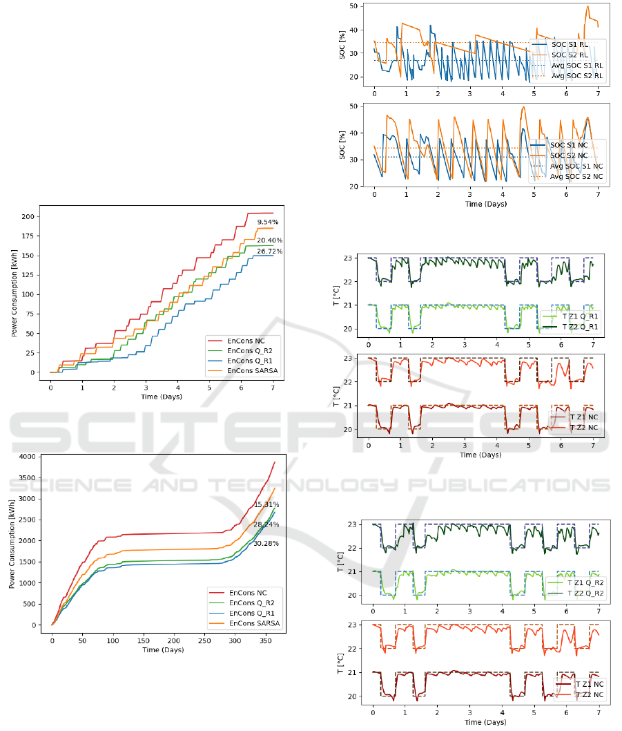
storage tanks. Figure 9 shows that the average charge
level of the thermal storage tank
and
ist for
exmaple under Q-learning 26.88% and 30.01%, while
without RL algorithm, namely with the normal
control this argument is 34.44% and 33.94%,
respectively.
In addition, the indoor temperature in the two-
zone building under RL and NC approaches are
illustrated in Fig. 10 - Fig. 12. We can see that our RL
approaches ensures that the presets thermal comfort
level is maintained and the difference between set
point and actual temperature is minimal.
Figure 7: Comparison of total electrical Consumption one
week.
Figure 8: Comparison of total electrical consumption over
the year.
Figure 9: State of charge in
and
.
Figure 10: Temperature in zone 1 and zone 2 (Q_R1 vs.
NC).
Figure 11: Temperature in zone 1 and zone 2 (Q_R2 vs.
NC).
SMARTGREENS 2021 - 10th International Conference on Smart Cities and Green ICT Systems
64
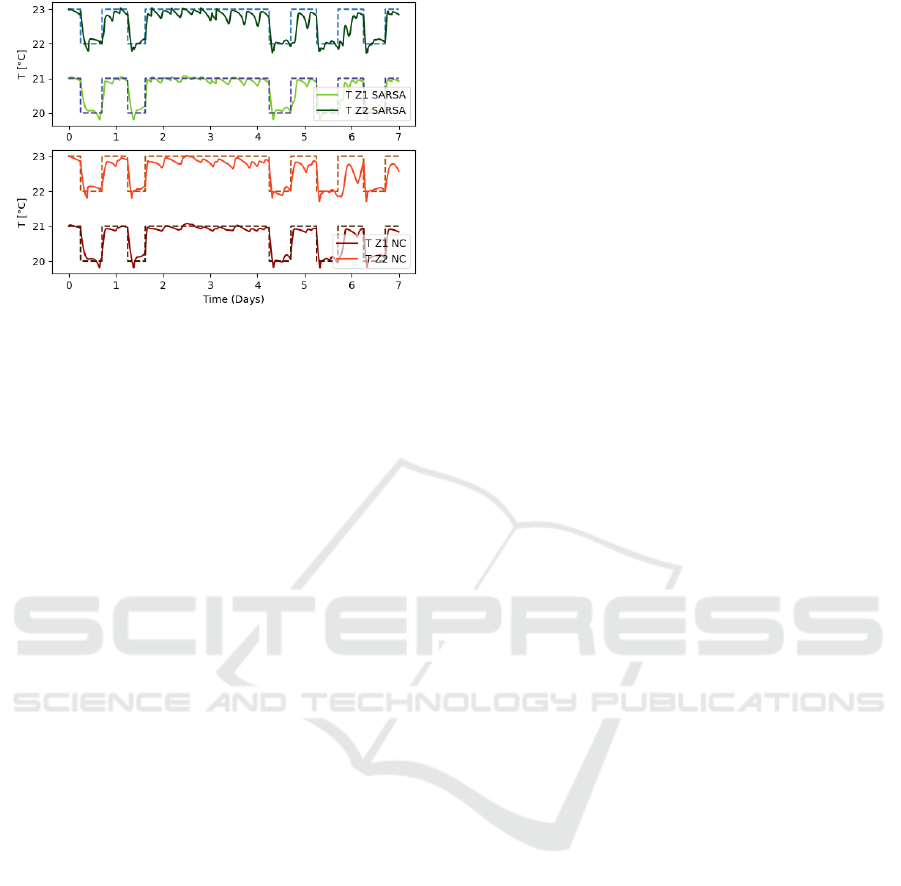
Figure 12: Temperature in zone 1 and zone 2 (SARSA vs.
NC).
6 CONCLUSION
The simulation results presented in the sections above
show that both control approaches MPC as well as RL
are able to provide acceptable output for the energy
manager. Both are capable of saving energy while
maintaining comfort compared to the standard control
algorithms. In particular, RL achieved better results.
Compared to the results presented in (Seidel and
Huang, 2020) the performance of the RL was
improved. Further, compared with the successful
applications of RL to home management systems
mentioned from Mason, K. (Mason and Grijalva,
2019), our result of electrical energy saving are in
accordance with the results from other researches.
In case of MPC, the heuristic optimisation method
which is suited to this kind of discrete problems
require much computational effort in order to get
close to the optimal solution. Thus, corresponding
resources such as powerful PC hardware are required.
If the energy system grows and new system
components or functions are added, the optimisation
task would also become increasingly complex to
solve. Further investigations are therefore needed to
ensure the real-time capability of this control
algorithms and to improve the cost-benefit ratio.
In contrast, RL with Q-table requires a learning
phase before being commissioned as EM. During the
online operation phase the required resources are
relatively low and real-time capability is not critical
since no simulation runs are required. Therefore, for
the presented task of the energy manager, RL
algorithm is a much more attractive approach.
However, implementing the RL agent and especially
the tuning of the hyperparameters during the learning
phase is not straightforward. Thus, strategies for
setting the optimal hyperparameters need to be
analysed in future works.
On the other hand, the teaching of the RL agent
with the aforementioned models can be processed
offline. Learning can also be continued during
operation with sensor data from the real energy
system so that an adaptation of the RL agents
behaviour to the real energy system can be achieved
and thus, further improvements of the results are
possible. However, real-world learning must be done
much more carefully since exploring new state-action
combination could result in discomfort or waste of
energy.
On the contrary, in case of MPC, a change within
the energy system would require an adaption of the
prediction model in order to obtain optimal results.
Otherwise the output of the energy manager may not
be acceptable. However, in order to achieve very
good results right at the beginning of operation phase,
an accurate system model is indispensable for both
MPC and RL.
Another important difference between the two
methods is the weighting of long-term gains. For the
classic MPC optimisation, the time horizon in which
an optimal solution must be found is fixed in general.
The actions and the cost at each time step within the
time horizon are equally weighted. For RL, the profit
of the next action step has the biggest impact, while
profits of future actions are weighted less according
to the discount factor. Therefore the greater
uncertainty of long-term forecasts can be taken into
account.
In this paper, Q-Learning yields very good results
for the energy system. In case of more complex
systems and control tasks, it may be necessary to use
more advanced methods of RL, such as deep learning
with neural networks, which require much more
training. For Q-tables, however, a few hundred
episodes are sufficient to achieve good control
results.
7 SUMMARY AND OUTLOOK
Classic MPC and RL were tested and compared for
the high-level control of the energy system of a
single-family house. In this paper RL can achieve
better results than MPC with much less computational
resources and is therefore suited for the online control
of the building energy system.
Reinforcement learning thus offers attractive
possibilities which the authors will continue to
analyse in future works.
Energy Optimal Control of a Multivalent Building Energy System using Machine Learning
65

Moreover, we will take a deeper look at the
optimization problem itself and especially the
potential of multi-objective optimisation in the
context of RL and MPC, since for complex energy
systems, different and more conflicting goals will
arise.
REFERENCES
Bundesministerium für Wirtschaft und Energie (BMWi).
(2019). Energieeffizienz in Zahlen.
Renaldi, R., Kiprakis, A., Friedrich, D., 2017. An
optimisation framework for thermal energy storage
integration in a residential heat pump heating system.
In Applied Energy 186, 520–529.
Oldewurtel, F., Parisio, A., Colin, N. J., et al., 2012. Use of
model predictive control and weather forecasts for
energy efficient building climate control. In Energy and
Buildings 45, 15–27.
Chen, Y., Norford, L. K., Samuelson, H. W., et al., 2018.
Optimal control of HVAC and window systems for
natural ventilation through reinforcement learning. In
Energy and Buildings 169, 195 – 205.
Mason, K., Grijalva, S., 2019. A Review of Reinforcement
Learning for Autonomous Building Energy
Management. In Computers & Electrical Engineering
78, 300-312.
Palensky, P., Dietrich, D., 2011. Demand Side
Management: Demand Response, Intelligent Energy
Systems, and Smart Loads. In: IEEE Trans. Ind. Inf. 7
(3), S. 381–388.
Paschke, F., Franke, M., Haufe, J., 2016. Modell-prädiktive
Einzelraumregelung auf Basis empirischer Modelle, In
Central European Symposium on Building Physics
2016 / Bausim 2016.
Paschke, F., 2020. PEM-Identification of a block-oriented
nonlinear stochastic model with application to room
temperature modeling, In 28th Mediterranean
Conference on Control and Automation (MED2020),
2020, 351-356.
Blochwitz, T., Otter, M., Arnold, M., Bausch, C., Clauss,
C., Elmqvist, H., et al., 2011. The Functional Mockup
Interface for Tool independent Exchange of Simulation
Models. In Proceedings 8th Modelica Conf., 105-114.
Dassault Systems, 2017. Fmpy. URL: https://git
hub.com/CATIA-Systems/FMPy, last access 2.5.2020.
Mynttinen, I., Hoffmann, A., Runge, E., Li, P., 2015.
Smoothing and regularization strategies for
optimization of hybrid dynamic systems. In: Optim Eng
16 (3), S. 541–569.
Wigstrom, O., Lennartson, B., 2012. Scheduling model for
systems with complex alternative behaviour. In 2012
IEEE International Conference on Automation Science
and Engineering (CASE), 587–593.
Wigström, O., Lennartson, B., 2014. An Integrated CP/OR
Method for Optimal Control of Modular Hybrid
Systems. In: IFAC Proceedings Volumes 47 (2), S.
485–491. DOI: 10.3182/20140514-3-FR-4046.00130.
Schlüter, M., Egea, J. A., Bangam J. R., 2009: Extended
ant colony optimization for non-convex mixed integer
nonlinear programming. In: Computers & Operations
Research 36 (7), S. 2217–2229
Jordan, M. I., & Mitchell, T. M., 2015. Machine learning:
Trends, perspectives, and prospects. In Science,
349(6245), 255-260.
Sutton, R. S., & Barto, A. G., 2018. Reinforcement
learning: An introduction. MIT press.
Gao, G., Li, J., & Wen, Y., 2019. Energy-efficient thermal
comfort control in smart buildings via deep
reinforcement learning. In arXiv preprint
arXiv:1901.04693.
Szepesvári, C., 2010. Algorithms for reinforcement
learning. In Synthesis lectures on artificial intelligence
and machine learning, 4(1), 1-103.
Mason, K., & Grijalva, S., 2019. A review of reinforcement
learning for autonomous building energy management.
In Computers & Electrical Engineering, 78, 300-312.
Seidel, S., Huang, C., Mayer, D., et al., 2020,
Kostenoptimale Steuerung eines multivaltenten
Gebäudeenergiesystems mittels modellprädiktivem
Ansatz und Reinforcement Learning, In AUTMATION
2020 – 21. Leitkongress der Mess- und Automa-
tisierungstechnik, VDI-Berichte 2375, 43-56.
Seidel, S., Clauß, C., Majetta, K., et al., 2015, Modelica
based design and optimisation of control systems for
solar heat systems and low energy buildings, In 11th
International Modelica Conference 2015. Proceedings :
Versailles, France, September 21-23, 2015, 401-410.
SMARTGREENS 2021 - 10th International Conference on Smart Cities and Green ICT Systems
66
