C*DynaConf: An Apache Cassandra Auto-tuning Tool for

Internet of Things Data

Lucas Benevides Dias

1 a

, Dennis S

avio Silva

2,4 b

, Rafael T. de Sousa Junior

3 c

and Maristela Holanda

2 d

Institute for Applied Economic Research, Bras

ılia, Brazil

Department of Computer Science, University of Bras

ılia, Bras

ılia, Brazil

Department of Electrical Engineering, University of Bras

ılia, Bras

ılia, Brazil

Federal University of Piau

ı, Picos, Piau

ı, Brazil

Keywords:

Databases, NoSQL, Internet of Things, Time Series, Auto-tuning, Cassandra, Compaction Strategies.

Abstract:

Internet of Things environments may generate massive volumes of time series data, with speciﬁc charac-

teristics that must be considered to facilitate its storage. The Apache Cassandra NoSQL database provides

compaction strategies that improve data pages’ organization, beneﬁting the storage and query performance for

time series data. This study exploits the temporal characteristics of IoT data, and proposes an engine called

C*DynaConf based on the TWCS (Time Window Compaction Strategy), which dynamically changes its com-

paction parameters according to conﬁgurations previously deﬁned as optimal, considering current metadata

and metrics from the database. The results show that the engine’s use brought a 4.52% average gain in

operations performed compared to a test case with optimal initial conﬁguration that changes the scenario’s

characteristics change over time.

1 INTRODUCTION

Internet of Things (IoT) sensor data can be classiﬁed

as a peculiar example of a time series and they have

speciﬁc features that can be exploited by the database

to improve its performance and reduce the require-

ments of storage space (Li et al., 2012; Savaglio et al.,

2019). These data are on a massive scale, they are

ordered and retrieved by the temporal key, have a

low frequency of update, and expire after a certain

time (Dias et al., 2018). Relational databases, in gen-

eral, are not the best ﬁt for storing massive data, es-

pecially coming from IoT applications (Zhu, 2015;

Vongsingthong and Smanchat, 2015). Some studies

point to NoSQL databases as a solution (Zhu, 2015;

Oliveira et al., 2015; Kiraz and To

gay, 2017).

To improve the data organization, NoSQL

databases must have compaction strategies for their

data pages. This operation reads and merges the data

pages on disk resulting in a new page (Ghosh et al.,

https://orcid.org/0000-0001-5316-877X

https://orcid.org/0000-0002-1613-4922

https://orcid.org/0000-0003-1101-3029

https://orcid.org/0000-0002-0883-2579

2015). It also allows the sequential reading and writ-

ing of data, which is more efﬁcient than manipulat-

ing fragmented data (Kona, 2016). Furthermore, the

compaction strategies deallocate the space reserved

for deleted data (Warlo, 2018).

The Apache Cassandra database derived the com-

paction functionality from BigTable (Wu et al., 2018).

The conﬁguration of the parameters that deﬁne the be-

havior of Cassandra’s compaction strategies is deﬁned

before the execution and performed manually. How-

ever, it is challenging for users to manually manage

the strategy because they must know the most efﬁ-

cient settings in advance. An inappropriate conﬁgu-

ration can result in higher query response times and

lower throughput for the NoSQL database in IoT en-

vironments. An automatic conﬁguration mechanism

can therefore beneﬁt the system’s performance and

usability.

This paper aims to present the C*DynaConf, an

auto-tuning mechanism for the parameters of the Cas-

sandra database’s compaction strategy, focused on

IoT data, which seeks to maximize the throughput and

minimize the response time. The C*DynaConf must

change the system settings according to the relation

between reading and writing operations and the data’s

Dias, L., Silva, D., Sousa Junior, R. and Holanda, M.

C*DynaConf: An Apache Cassandra Auto-tuning Tool for Internet of Things Data.

DOI: 10.5220/0010476000920102

In Proceedings of the 6th International Conference on Internet of Things, Big Data and Security (IoTBDS 2021), pages 92-102

ISBN: 978-989-758-504-3

lifetime.

The rest of this paper is organized as follows: Sec-

tion 2 presents the theoretical background and re-

views the related work. Then, Section 3 describes

the C*DynaConf auto-tuning mechanism. Section 4

introduces the execution environment, its conﬁgura-

tions, and details about the test cases. Section 5 brings

the analysis of the results. Section 6 concludes and

considers future works.

2 THEORETICAL BACKGROUND

The Apache Cassandra is one of the most popular

NoSQL databases (Gujral et al., 2018). Some of its

characteristics make it suitable for the storage of IoT

data. It supports high data insertion rates and avail-

ability (Wu et al., 2018), has a data model adequate

to sequential data regardless of type and size (Lu and

Xiaohui, 2016), uses data compaction strategies that

exploit the characteristics of IoT-like data to improve

storage and management (Datastax, 2018), and has a

conﬁguration that limits the data TTL (time-to-live)

(Carpenter and Hewitt, 2016).

In Cassandra’s storage, data is stored in memory

in structures called Memtables and ﬂushed to the disk

when the Memtables reach their maximum size or

age (the difference between the current time and the

time when they were created), or by user command

(Ghosh et al., 2015). Once this data goes to the disk,

it is received persistently in structures called SSTa-

bles (Chang et al., 2008). They do not accept changes

and deletions, and their structures consist of ordered

arrays containing keys and values (Hegerfors, 2014).

The key used in SSTable arrays for searching and or-

dering is called the clustering key.

When a record in an SSTable is changed, the

new value is stored in a Memtable, and the previous

value, held in the SSTable, remains at it is. When the

database reads the altered data, it joins the Memtable

data to the SSTable data before displaying it to the

user (Eriksson, 2014). If a Memtable with data from

a changed record is ﬂushed on disk, there will be data

from this record in more than one SSTable, generat-

ing an access cost to two SSTables in the moment of

the reading. This gets worse as the changes in a single

record increase (Chang et al., 2008).

Moreover, the data deletion does not change the

Memtables or SSTAbles already stored. A logical

deletion occurs – that is, a null ﬂag is added to the

deleted cell – in a new MemTable. The cell or row

excluded is called tombstone (Carpenter and Hewitt,

2016). The data deleted from Cassandra receive a pa-

rameter called a grace period, representing the min-

imal time needed to delete the data. However, the

deﬁnitive exclusion of deleted data does not occur au-

tomatically when the tombstone reaches the grace pe-

riod. The data deallocation and recovery of the disk

space only happen with the SSTable compaction.

When a record passes through many changes,

there will be many versions of it in the database,

spread on different disk pages. The database period-

ically must perform an operation called compaction,

which merges these disk pages into new ones through

a merge-sort algorithm (Ghosh et al., 2015). This

operation should not be mistaken with algorithms

for data compression and compaction. In this com-

paction, insertions and upsertions that changed the

same data are discarded, leaving only the most re-

cent operation, with the most up-to-date version of

the data. The compaction operation has a cost, but it

is worthwhile because the subsequent read operations

become faster.

Different compaction strategies deﬁne what pages

must be merged and the moment when this must

occur (Lu and Xiaohui, 2016). The objectives of

these strategies in Cassandra are to allow the NoSQL

databases to access fewer SSTables to read data and

to use less disk space (Hegerfors, 2014; Ghosh et al.,

2015; Eriksson, 2014; Apache Software Foundation,

2020).

Among Cassandra’s compaction strategies, the

TWCS (Time Window Compaction Strategy) stands

out for managing IoT-like data (Jirsa and Eriksson,

2016; Apache Software Foundation, 2020). It ex-

ploits the characteristics of time-series data and uses

time-window-based compaction. Data inserted in the

same time-window stay together and contiguously be-

cause they have more chance of being retrieved to-

gether. Some TWCS parameters are relevant to this

work. The compaction window size deﬁnes the

time window size in which the SSTables will be com-

pacted. The compaction window unit is the time

unit (minutes, hours, or days) (Jirsa and Eriksson,

2016). The min threshold and max threshold pa-

rameters deﬁne, respectively, the minimal and max-

imum number of SSTables in disk needed to start a

compaction operation.

The TWCS performs the compaction considering

the adjacency between pages, being adequate to store

IoT data, commonly inserted in contiguous time inter-

vals. This means that if disordered insertions do not

occur, only one data page in the disk will have the data

at a speciﬁc moment. Thereafter time interval queries

require fewer disk pages to be accessed. Because of

these advantages, this proposal uses the TWCS strat-

egy.

C*DynaConf: An Apache Cassandra Auto-tuning Tool for Internet of Things Data

2.1 Related Works

Among the studies related to auto-tuning in databases,

few are dedicated to the conﬁguration of compaction

strategies since it is a speciﬁc problem of some

NoSQL databases. Sathvik (2016) analyzed Cassan-

dra’s performance, changing the conﬁguration of the

Memtables and a table called Key-Cache, which re-

sides in memory and stores pointers to retrieve the

SSTable data swiftly. However, the study does not an-

alyze the performance after changing the compaction

strategy parameters, neither studies IoT scenarios.

In Lu and Xiaohui (2016), stress scenarios were

executed, and metrics were analyzed. It was con-

cluded that the DTCS (Date-Tiered Compaction Strat-

egy) is adequate for use with time series, resulting

in better performance when compared to other com-

paction strategies available in Cassandra.

Kona (2016) investigates, using Cassandra, met-

rics related to the performance of compaction met-

rics. This work compares the strategies DTCS, STCS

(Size-Tiered Compaction Strategy), and LCS (Lev-

eled Compaction Strategy) in an intensive writing en-

vironment. It is concluded that the DTCS strategy is

not the best for the simulated scenario, losing in per-

formance to the LCS. However, in the analyzed case,

the data does not have the characteristics of a time-

series. It is worth mentioning that the DTCS strategy

is deprecated, and the TWCS replaced it.

Ravu (2016) simulated Cassandra’s behavior in

three workload situations, one write-intensive, one

read-intensive, and one balanced, with the same num-

ber of readings and writings. The DTCS strategy pre-

sented better results for the read-intensive workload,

even though the data does not have time-series char-

acteristics. For the write-intensive scenario, the LCS

strategy showed a better performance. At the time of

publication, the TWCS strategy was not available for

Cassandra yet.

In Xiong et al. (2017), positive results were ob-

tained with the HBase NoSQL database’s auto-tuning.

Ensemble learning algorithms were used to reach an

optimal conﬁguration. Twenty-three conﬁguration

parameters were analyzed in ﬁve speciﬁc scenarios,

and the parameters with a higher impact on the per-

formance were identiﬁed. The auto-tuning compo-

nent increased the throughput by 41% and reduced

the latency by 11%. However, works similar to this

were not found using Cassandra, and none of the ﬁve

scenarios had speciﬁc IoT characteristics.

Katiki Reddy (2020) proposes a new Random

Compaction Strategy (RCS), that improves the efﬁ-

ciency of compaction, when compared to LCS and

STCS, in some scenarios, at a rate of 4 to 5 percent in

latency and operations per second. However, the sce-

narios were not IoT speciﬁc and were not compared

with the main strategy used in this article, which is

TWCS. Moreover, this new strategy has not been

adopted by the Cassandra community.

Table 1 summarizes the related works. None of

the related works implements an auto-tuning tool for

the Cassandra NoSQL database; neither are speciﬁc

for IoT data. Differently of them, our paper proposes

C*DynaConf, an auto-tuning software for IoT data

in NoSQL Cassandra database, which simpliﬁes the

use of database compaction strategies, abstracting the

complexity of some parameters.

Table 1: Related Works.

Related Paper NoSQL Strategy

Sathvik (2016) Cassandra Does not apply

Lu and Xiaohui (2016) Cassandra DTCS, STCS

and LCS

Kona (2016) Cassandra DTCS, STCS

and LCS

Ravu (2016) Cassandra DTCS, STCS

and LCS

Xiong et al. (2017) HBase Does not apply

Katiki Reddy (2020) Cassandra RCS

3 C*DynaConf

C*DynaConf is auto-tuning software based on pre-

deﬁned rules. It uses a table that stores the opti-

mal conﬁguration points previously known. Based

on these points and the metadata obtained from the

database, it computes and applies near-optimal val-

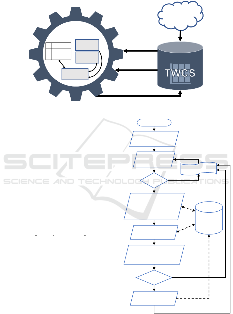
ues for Cassandra’s compaction parameters. Figure

1 shows the C*DynaConf architecture. The meta-

data search component is responsible for reading the

column families’ settings conﬁgured with the TWCS

strategy in Cassandra and passing them to the pa-

rameter calculator. The retrieved metadata are the

compaction window size, the min threshold and

the TTL of the column family.

The metrics search component requests from Cas-

sandra the metrics that it uses to check the ratio be-

tween readings and writings for the column family

receiving the auto-tuning. C*DynaConf has a timer

that iterates its main routine execution every 30 sec-

onds. This frequency was chosen because it is suf-

ﬁcient to subsidize the conﬁguration without burden-

ing the database performance. The parameter calcu-

lator considers the metadata received and the metrics,

calculates the optimal points according to a table of

predeﬁned optimal conﬁguration points and compares

them to the table’s parameters. If the optimal conﬁgu-

ration is not set on the table, the program changes the

IoTBDS 2021 - 6th International Conference on Internet of Things, Big Data and Security

Cassandra

TWCS

C*DynaConf

Metadata

Searcher

Metrics

Searcher

Parameters

Calculator

Table

Optimal

Points

IoT

Tables Metadata

JMX Metrics

Apply new parameters

Figure 1: C*DynaConf Architecture Diagram.

table settings with the new parameters.

C*DynaConf uses the TWCS compaction strat-

egy. It is developed in Java and uses some com-

ponents to simplify its construction. The Java

connection driver for Cassandra was developed by

DataStax

, which manages the connection to the

cluster nodes (DataStax, 2018). Another package

used is the Criteo Cassandra Exporter (Criteo, 2018),

which manages the metrics received through JMX and

carries out pre-computing to populate objects with

metrics deﬁned in conﬁguration ﬁles.

Figure 2 presents the C*DynaConf ﬂowchart. The

program starts receiving, through the command line,

the Keyspace k that must be monitored and the

name of some node of the cluster c. Afterwards,

C*DynaConf starts a loop – that is interrupted only

by the user – on which it veriﬁes if there are col-

umn families with the TWCS strategy conﬁgured and,

if so, retrieves their metadata, from which are used

the compaction window size, the min threshold,

and the table TTL. Later, the mechanism will search

the metrics of the number of read and write opera-

tions, to deﬁne the proportion among them. Then, the

program calculates what scenario of optimal points is

closest to the execution environment. The table meta-

data is compared to the optimal conﬁguration values

and changed if different through an ALTER TABLE

command. There is then a 30 second pause, and the

loop repeats.

3.1 Read/Write Ratio Metric

C*DynaConf changes the TWCS parameters accord-

ing to variations on the TTL and the proportion be-

tween reading and writing operations. The ﬁrst is ob-

Start (c, k)

Connect to Cluster c,

on Keyspace k

Search tables

with TWCS

Found?

Search for metadata:

compaction window size,

min threshold, table TTL

Search for metrics

Check if the configuration

conforms to the optimal

points

Wait 30 seconds

Is optimal?

Cassandra

Apply optimal

configuration

Yes

Figure 2: Data Flow Diagram for C*DynaConf.

C*DynaConf: An Apache Cassandra Auto-tuning Tool for Internet of Things Data

tained from the table’s metadata. But the ratio must be

calculated based on metrics obtained from the cluster

nodes.

There is a set of metrics that measures the client

requests, called ClientRequest. In this set, there is a

Java object called Meter, that stores the read and write

metrics and the throughput of the second in execution,

and also an exponential weighted moving mean that

represents the mean values from the last 1, 5, and 15

minutes (Apache Software Foundation, 2016). The

exponential weighted moving mean is calculated, as-

signing higher weights to the most recently observed

measurements.

These metrics contain a history of the last minutes,

already summarized. If the program considers only

the throughput value of the moment when the meta-

data is searched, it would be subject to oscillations

from other sources, for example, pauses of the JVM

for Garbage Collection. The frequency of compaction

parameter changing would be much higher, increas-

ing the costs. The mean value of the last 5 minutes

was chosen because this value is enough to perceive

changes in the characteristics of an IoT environment.

The read metric ClientRequest.Read.Latency.

FiveMinuteRate

and the write metric ClientRe-

quest.Write.Latency.FiveMinuteRate proved to be re-

liable during the experiments, representing the pro-

portion values as deﬁned in the Cassandra Stress

Tool. These metrics are present in all nodes. Since

they are retrieved only every 30 seconds, the program

queries all nodes and add the reading and writing

taxes, and then calculates the proportion of readings.

This metric has a limitation. It is deﬁned at server

level, that is, it is not speciﬁc to a certain table or

keyspace. Thus, its reliability as an indicator depends

on Cassandra receiving only requests for manipulat-

ing monitored tables. During the tests performed in

this research, the Cassandra Stress Tool only gener-

ated workload for one column family at a time.

4 EXECUTION ENVIRONMENT

The tests were executed in a cluster with ten virtual

machines with the same capacity: a core of the Intel

Xeon

processor; magnetic hard disks of 7200 rpm,

with 50GB of space; 3.2GB of RAM DDR3 memory;

and Gigabit Ethernet interface. Besides the ten cluster

nodes, an extra computer was employed for data gen-

eration and loading into the Cassandra cluster. This

node contains 40GB of disk space, one core of the

Despite having latency in the name, this metric mea-

sures the throughput.

Intel Xeon

processor, and 2GB of RAM. All nodes

used the Ubuntu Linux version 16.04 as the operating

system, and Cassandra database version 3.11.1.

Some default conﬁgurations of Cassandra were

modiﬁed. The write timeout values were doubled, and

the reading timeout was increased ﬁvefold. This was

necessary due to the high work level and low process-

ing and I/O power of the hardware available. More-

over, some parameters were modiﬁed to allow the

client to connect to different nodes via JMX to mon-

itor metrics, a feature not enabled by default. In the

keyspace conﬁguration, the replication strategy em-

ployed was the SimpleStrategy, and the replication

factor was three.

Simulated data with IoT characteristics were used

to perform the tests. A common aspect of IoT data is

that they expire, and in all scenarios, the executions

enabled the parameter TTL in the column family. Ac-

cording to the chosen scenarios, the TTL varied be-

tween one and three hours. The grace period was de-

ﬁned as 1800 seconds for all executions.

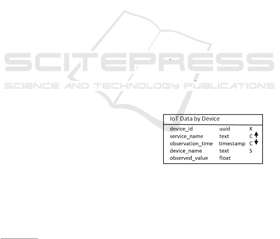
Figure 3 presents the data model in the Chebotko

notation (Chebotko et al., 2015). A universal unique

identiﬁer type that identiﬁes a sensor device was

chosen as partition key. There can be many mea-

suring services for every device, represented in the

service name ﬁeld. In all scenarios tested in this

study, there is a ﬁxed number of ﬁve services for each

sensor, which means ﬁve time-series for every device.

The observation time receives decreasing index-

ing because most recent data is more usually queried

and retrieved. The remaining ﬁelds receive the device

name and value, with the float type.

Figure 3: Column Family Scheme.

An IoT environment often performs more writings

than readings, and during the tests, we varied the read-

ing percentage from 1% to 30% of the total of opera-

tions. Three queries were deﬁned in CQL (Cassandra

Query Language):

devdat: retrieves all data emitted by a certain de-

vice, passing its identiﬁer. It is responsible for 40% of

the reading operations sent to the database during the

executions. This query has a limiter to retrieve 500

rows at most.

IoTBDS 2021 - 6th International Conference on Internet of Things, Big Data and Security

SELECT * FROM iot_data

WHERE device_id = ?

LIMIT 500

lesrow: retrieves data from a speciﬁc time series,

passing as a parameter the device identiﬁer and the

series name. It is responsible for 30% of the queries

and has a 500 rows limiter.

SELECT * FROM iot_data

WHERE device_id = ? AND service_name = ?

LIMIT 500

avgdat: calculates the average of the values observed

by a device measurement. Returns only one line, al-

though covering all registers in the database. It is re-

sponsible for 30% of the stress tool’s queries sent to

the database.

SELECT device_id, AVG(observed_value)

FROM iot_data

WHERE device_id = ? AND service_name = ?

Cassandra has an open-source tool called Cassandra-

Stress tool, capable of generating a pool of tests, with

the functionality of choosing the statistic distribution,

mean, and standard deviation of the generated data.

Version 4.0 of the tool was used and its code was

adapted speciﬁcally for the tests. It has several user

modes, and the one chosen , has the user inputting the

conﬁgurations through a YAML ﬁle. This ﬁle con-

tains the column family’s scheme and the value distri-

bution of every column. At this point, it is deﬁned that

every device generates ﬁve time series, and, at each

operation, 60 values are inserted in every time series.

The queries are also deﬁned in the ﬁle. All YAML

conﬁguration ﬁles are available in (Dias, 2018).

The Cassandra-stress tool is multithread. It ex-

ecutes the same task with an increasing number of

threads, up to the point that there are two simulations

with a higher number of threads, on which they had a

loss of performance. In the initial stage of the tests,

some numbers of threads were tested for IoT data

reading and writing operations. The optimal through-

put value was reached with 24 threads in all prelimi-

nary tests, and this number of threads was used during

the research.

When executing the stress tool, it was decided to

run the stress process limited by time, using the pa-

rameter duration expressed in minutes. The opera-

tion ﬁnishes exactly when the deﬁned time is reached.

This way, an execution with better conﬁguration will

perform a higher number of operations.

The Cassandra-stress tool generates a log ﬁle that

contains values collected in intervals of 30 seconds

and, at the end of the execution, presents a consoli-

dated mean of the throughput, latency, and other exe-

cution metrics of the JVM’s Garbage Collector. Cas-

sandra provides metrics for performance evaluation.

Every node in the cluster generates its metrics, allow-

ing an individual evaluation, but they must be consoli-

dated for an integral assessment of the system. During

the research, two methods were used to retrieve the

metrics. One along the operation observation, to per-

form the database tuning and obtain optimal conﬁg-

uration points for the compaction strategy, and other

during the D*DynaConf operation.

It is not convenient for the proposed software to

read ﬁles in different network nodes. It can become

a costly task and demand ﬁle sharing for all nodes,

which means extra workload in a production environ-

ment. Instead of reading in the disk, C*DynaConf

captures the metrics through the connection driver,

using the JMX protocol. The metrics are the same,

but the method of retrieving them is different. The

periodicity on which C*DynaConf works is also 30

seconds. Therefore, the most used metrics along the

process were:

• Throughput: number of operations by second.

• Latency: time needed for the database system to

answer a request.

• Disk Space: total number of bytes needed to store

the data.

• Execution Time: for a certain number of insertions

and queries to be performed, the most efﬁcient

conﬁguration is the one that ﬁnishes ﬁrst.

• Number of Touched Partitions: directly propor-

tional to the number of read and write operations

performed. The highest performing conﬁguration

is the one that touches more partitions in a speciﬁc

period.

Besides the metrics cited above, C*DynaConf also

uses two exponentially weighted moving averages,

called ClientRequest.Read.Latency.FiveMinuteRate

and ClientRequest.Write.Latency.FiveMinuteRate.

4.1 Simulated IoT Scenario

To evaluate the effects of using C*DynaConf, it was

modeled a scenario where the variables observed by

the program change (Figure 4). These variables are

the TTL and the ratio between readings and writings.

An example that can illustrate the simulated sce-

nario is one of a smart city, with a ﬁxed number of

sensors, at night. The control center would have as

the standard conﬁguration the 1 hour TTL and, in

the evening, conditions are the same as in daytime:

the reading operations made by people are responsi-

ble by 10% of the operations. As the night falls, the

operation team would be reduced and, therefore, data

would need a bigger TTL, so that it could be read by a

C*DynaConf: An Apache Cassandra Auto-tuning Tool for Internet of Things Data

remote response team, before expiring. Moreover, at

this stage, Decision Support Systems would read and

load the Data Warehouses, raising the reading propor-

tion for 30%. In the third stage, which would start at

1 AM, monitoring would be made only by computers

and people would be paged only in case of some inci-

dent. At late night, the TTL would be of 3h in order

to the incident response team have enough time to be

ready and go to the control center, before data get ex-

pired. Over the late night, reading operations would

be done only by monitoring tools, and so the reading

proportion would be reduced do 3%. At dawn, the

daylight conditions would be resumed, just like stage

The simulated scenario has four stages, the ﬁrst

and the last being equal. They have a TTL deﬁned

in 1h, a duration of 150 minutes and the proportion

of 90% writings and 10% readings. The second stage

takes 200 minutes, has TTL deﬁned as 2h, and 30%

of the operations are readings. The third stage lasts

300 minutes, has a TTL of 3h and 3% of readings.

The experiments checked whether the auto-tuning

mechanism could generate a better scenario than a

manual conﬁguration, even if this manual conﬁgura-

tion equals a conﬁguration considered optimal before

the environment changes. The initial stage is conﬁg-

ured with the optimal parameters found at the tuning

step. The environment then changes its TTL condi-

tions and the ratio between write and read operations.

In the last stage, the initial conditions are used again.

4.2 Tuning of the TWCS Strategy

Some previous experiments were performed to ad-

just the TWCS strategy parameters to optimal perfor-

mance settings and support creating the C*DynaConf

auto-tuning component.

The compaction window size is the main

TWCS parameter and one of the variables considered

by C*DynaConf auto-tuning component. After the

compaction period, SSTables are not compacted by

TWCS anymore. Its minimum value is 1 minute, and

in this study, an interval from 1 to 80 minutes was

investigated in the experiments because, in prelimi-

nary tests, improvements were not observed after this

limit. Several tests were performed to ﬁnd the op-

timal points, i.e., the settings with better results for

some conﬁguration, changing the TTL, and the ra-

tio between readings and writings. The conﬁgurations

were analyzed considering the throughput, the mean

latency – mean response time between all the reading

and writing operations – and the number of touched

partitions. Table 2 summarizes the optimal points for

the C*DynaConf execution.

Table 2: Compaction Window Size - Optimal points (min-

utes).

Scenarios TTL 1h TTL 2h TTL 3h

Reading 3% 2 12 35

Reading 10% 10 10 25

Reading 30% 22 35 60

Simulations were performed to ﬁnd the most suitable

conﬁgurations for the min threshold, which default

value is 4, varying the values from 2 to 14 in a sce-

nario where 10% of the operations are readings. The

optimal values for min threshold, which will be ap-

plied in C*DynaConf, are: 6 when the TTL is set as

one hour, 8 when set as two hours, and 10 for a TTL

of three hours.

5 ANALYSIS OF THE RESULTS

The tests were executed three times with the static

conﬁguration – without using C*DynaConf – to mit-

igate oscillations from the computing environment,

which is not isolated. The column family was cre-

ated with the initial conﬁguration deﬁned as optimal

in the tuning of the strategy. That is, the compaction

window size was deﬁned as 10 minutes, and the min

threshold was deﬁned as 6. Later, the scenario con-

ﬁgurations changed, but the conﬁguration did not.

The tests using C*DynaConf were executed ﬁve

times. Similarly, in the static execution, the table was

created with the optimal values found during the ex-

ecutions described in Section 4.2. The average of the

three executions in the static scenario was calculated,

as well as the ﬁve executions using C*DynaConf.

This average is signiﬁcant because the standard de-

viation of the number of partitions touched was less

than 2% of the mean, in both cases, being of 1.58% in

the static conﬁguration, and 1.92% with the dynamic

conﬁguration. Along the execution, the C*DynaConf

scenario touched 4.52% more partitions than the static

scenario, evidencing the efﬁciency of the auto-tuning

mechanism against a static conﬁguration, even though

this static conﬁguration is set to an optimal point.

It must be considered that, from the 800 minutes

of the execution scenario, 300 are executed with the

optimal conﬁguration by the static conﬁguration. This

happened because, of the four stages, the ﬁrst and the

last, both with the duration of 150m, are equal and

the initial scenario is conﬁgured according to optimal

points previously simulated. Table 3 shows the av-

erage number of partitions touched during the execu-

tions with static and dynamic conﬁguration. When

considering only the scenarios where a conﬁguration

IoTBDS 2021 - 6th International Conference on Internet of Things, Big Data and Security

TTL 1h, 10% Reads TTL 2h, 30% Reads TTL 3h, 30% Reads TTL 1h, 10% Reads

150 min 200 min 300 min 150 min

0 150 min 350 min 650 min 800 min

18h10min 20h40min 0h 5h 7h30min

Figure 4: C*DynaConf Test Scenario.

change occurred, the improvement reaches 9.12% in

the number of touched partitions.

Table 3: Average of Partitions Touched by Stage.

Stage Conﬁguration Static Dynamic Gain

1 TTL 1h, 10% Reads 1.247.113 1.230.392 -1,34%

2 TTL 2h, 30% Reads 1.278.766 1.386.875 8,45%

3 TTL 3h, 3% Reads 2.022.161 2.215.174 9,54%

4 TTL 1h, 10% Reads 1.164.596 1.138.618 -2,23%

Total 5.712.636 5.971.059 4,52%

Since the number of touched partitions was higher us-

ing C*DynaConf, an improvement in the throughput

when using the mechanism is expected. The execu-

tion with the throughput closest to the average in ev-

ery group — with and without the auto-tuning – was

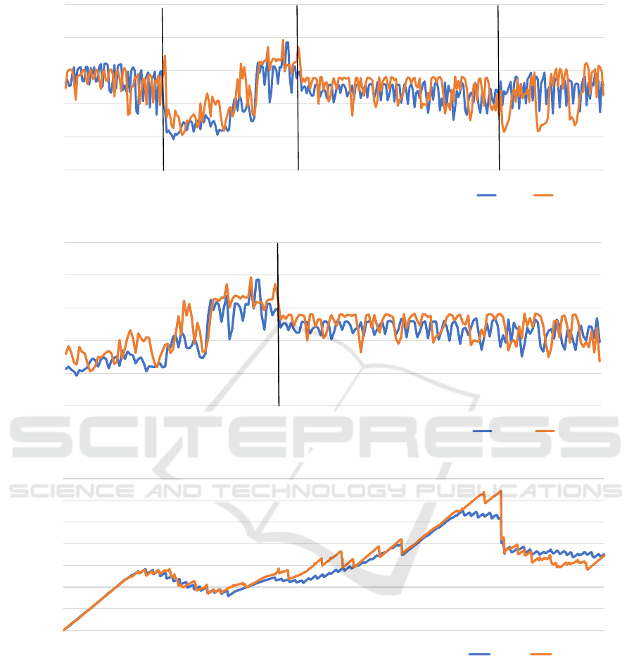
chosen to illustrate this behavior. Since the through-

put oscillates abruptly, the moving means with period

5 was used to smooth the curves, shown in Figure 5.

In Figure 5, the scenario’s stages are divided by

a black line. It can be perceived that the execu-

tion with dynamic conﬁguration has higher through-

put in stages 2 and 3, where the conﬁguration differ-

ence with the optimal points of compaction window

size and min threshold resulted in better perfor-

mance.

To better evaluate the stages of the scenario with

distinct parameter conﬁgurations, a section of the

curves of Figure 5 is presented in Figure 6. In these

two stages, an improvement of 9.3% in the execution

throughput when using C*DynaConf was perceived.

Regarding the latency, the execution with

C*DynaConf also performed better than the execution

of the static conﬁguration. The execution latency for

every conﬁguration is presented in Table 4. In the ex-

ecutions with the number of touched partitions closest

to the mean, the dynamic conﬁguration latency had a

4.09% lower latency.

Table 4: Average Latency (ms).

Stage Static Dynamic Gain

1 183,4 185,4 -1,09%

2 238,0 220,1 7,10%

3 189,4 172,1 9,13%

4 185,6 188,6 -1,62%

Total 199,7 191,6 4,09%

The latency also indicates another beneﬁt for the en-

vironment using C*DynaConf. In contrast, the same

can not be said about the disk space, presented in

Figure 7. The graphic represents an execution with

static conﬁguration and one with dynamic conﬁgura-

tion. The executions were chosen based on the num-

ber of touched partitions being closest to the mean.

In the ﬁrst execution stage, where the conﬁgura-

tions are the same, the space increases in a similar

way for both scenarios. Later, in the stage where the

reading operations changed to 30%, the stored space

decreases. Simultaneously, the inserted data start to

expire, and the insertion throughput does not provide

input data at the same rate as previously. In the third

stage, the TTL increases to 3h, and the disk volume

increases and reaches its peak shortly before the stage

changes. In the third stage, the dynamic conﬁguration

uses signiﬁcantly more space than the static conﬁgu-

ration.

Taking the average of used space along the 800

minutes of execution, the test with C*DynaConf used

3.6% more space than the static conﬁguration. How-

ever, the peak of used space – which can be consid-

ered the most relevant space indicator because it de-

termines the needed space – was 16.7% higher than in

the static environment. The conﬁguration with better

throughput and response time used more disk space.

This kind of permutation between storage space efﬁ-

ciency and response time performance is common to

computer science problems.

In the example scenario cited in 4.1 of a smart city,

the database server could afford an amount of 403.046

sensors collecting 5 observations each minute, using

C*DynaConf. This would represent an increase of

17.443 using the same database server, equivalent to

the database server used in the tests.

6 CONCLUSION

IoT environments can generate a high amount of data,

and the choice of storage mechanisms is critical to ob-

tain some value from this data. The rate of data cre-

ation can change over time because IoT environments

are often dynamic.

In this work, the C*DynaConf was developed.

C*DynaConf: An Apache Cassandra Auto-tuning Tool for Internet of Things Data

100

150

200

250

1 51 101 151 201 251 301 351 401 451 501 551 601 651 701 751

Throughput (ops/s)

Execution time (min)

Static C*DynaConf

Figure 5: Moving Means with 5 Periods of Throughput.

100

150

200

250

151 201 251 301 351 401 451 501 551 601

Throughput (ops/s)

Execution time (min)

Estático C*DynaConf

Figure 6: Moving Means of the Stages, with Different Parameters.

1 51 101 151 201 251 301 351 401 451 501 551 601 651 701 751

Disk space usage (GB)

Execution time (min)

Static C*DynaConf

Figure 7: Total Disk Space Used on the 10 Nodes, in GigaBytes.

This software allows the storage of IoT data in Cas-

sandra to be dynamic and have its conﬁgurations au-

tomatically adjusted according to some characteristics

of the received data. C*DynaConf conﬁgures, in real-

time and without manual intervention, the parameters

of TWCS. It reached a gain of 4.52% in the number

of performed operations in relation to the manual and

static conﬁguration. Its use must be avoided when the

limit in disk space is more critical than the response

time since C*DynaConf increased the need for disk

space by 16.7%. The parameter calculation consid-

ers the similarity to previously simulated scenarios.

If the execution environment differs from the simu-

lated environments, the beneﬁts to the performance

can be limited, or there can be some loss of perfor-

mance compared to a manual conﬁguration.

As future works, an auto-tuning tools based on ar-

tiﬁcial intelligence would be a great advance. This

work was based on static rules, that were previously

computed and do not evolve over time.

In addition, the tuning tests should be executed

in other computing environments, isolated from other

IoTBDS 2021 - 6th International Conference on Internet of Things, Big Data and Security

100

applications, and with hardware exclusively dedicated

to the tests. Cassandra has data compression features,

involving data compression algorithms to save disk

space. All tests performed in this work were per-

formed with the compression disabled in order not to

degrade the performance. Complimentary tests also

must be performed using compression algorithms to

verify the impact of this in the used disk space and re-

sponse time. The compaction and SSTable generation

operations involve many disk operations, which must

be affected by the SSTable fragmentation reﬂected

in the disk as a ﬁle. As future work, C*DynaConf

could check the node fragmentation level – i.e., the

number of ﬁle fragments – and, in case of high frag-

mentation, emit system calls to defragment the ﬁles.

Another possible improvement would be the use of a

real IoT dataset. The simulated data used in this work

was meant to reﬂect a natural environment. However,

the use of data generated in a production environment

should be used to validate the efﬁcacy and efﬁciency

of C*DynaConf.

REFERENCES

Apache Software Foundation (2016). Apache Cassan-

dra Monitoring. Available in http://cassandra.

apache.org/doc/latest/operating/metrics.html.

Acessed in 01/07/2021.

Apache Software Foundation (2020). Apache Cassan-

dra Compaction. Available in https://cassandra

.apache.org/doc/latest/operating/compaction/index.h-

tml?highlight=compaction%20strategies. Accessed

in 01/07/2021.

Carpenter, J. and Hewitt, E. (2016). Cassandra: The Deﬁni-

tive Guide: Distributed Data at Web Scale. ”O’Reilly

Media, Inc.”.

Chang, F., Dean, J., Ghemawat, S., Hsieh, W. C., Wallach,

D. A., Burrows, M., Chandra, T., Fikes, A., and Gru-

ber, R. E. (2008). Bigtable: A distributed storage sys-

tem for structured data. ACM Transactions on Com-

puter Systems (TOCS), 26(2):4.

Chebotko, A., Kashlev, A., and Lu, S. (2015). A big data

modeling methodology for apache cassandra. In 2015

IEEE International Congress on Big Data, pages 238–

245. IEEE.

Criteo (2018). cassandra exporter: Apache cassan-

dra® metrics exporter for Prometheus. Available

in https://github.com/criteo/cassandra exporter. Ac-

cessed in 01/07/2021.

Datastax (2018). Conﬁguring Compaction in Apache Cas-

sandra 3.0. Available in https://docs.datastax.com/

en/cassandra/3.0/cassandra/operations/opsConﬁgure

Compaction.html. Accessed in 01/07/2021.

DataStax (2018). Java Driver for Apache Cassandra -

Home. Available in https://docs.datastax.com/en/

developer/java-driver/3.5/. Accessed in 01/07/2021.

Dias, L. B. (2018). Github Repository: Experimental

data. Available in https://github.com/lucasbenevides/

mestrado. Acessado em 01/07/2021.

Dias, L. B., Holanda, M., Huacarpuma, R. C., and Jr, R.

T. d. S. (2018). NoSQL Database Performance Tun-

ing for IoT Data - Cassandra Case Study. In Proceed-

ings of the 3rd International Conference on Internet of

Things, Big Data and Security, pages 277–284, Fun-

chal, Portugal.

Eriksson, M. (2014). DateTieredCompactionStrategy :

Compaction for Time Series Data. Available in

http://www.datastax.com/dev/blog/datetieredcompac-

tionstrategy. Accessed in 01/07/2021.

Ghosh, M., Gupta, I., Gupta, S., and Kumar, N. (2015).

Fast Compaction Algorithms for NoSQL Databases.

In 2015 IEEE 35th International Conference on Dis-

tributed Computing Systems, pages 452–461.

Gujral, H., Sharma, A., and Kaur, P. (2018). Empir-

ical investigation of trends in nosql-based big-data

solutions in the last decade. In 2018 Eleventh In-

ternational Conference on Contemporary Computing

(IC3), pages 1–3. IEEE.

Hegerfors, B. (2014). Date-Tiered Com-

paction in Apache Cassandra. Available in

https://labs.spotify.com/2014/12/18/date-tiered-

compac- tion/. Acessed in 01/07/2021.

Jirsa, J. and Eriksson, M. (2016). Provide

an alternative to DTCS - ASF JIRA.

[CASSANDRA-9666]. Available in

https://issues.apache.org/jira/browse/CASSANDRA-9

666. Acessed in 01/07/2021.

Katiki Reddy, R. R. (2020). Improving Efﬁciency of

Data Compaction by Creating & Evaluating a Random

Compaction Strategy in Apache Cassandra. Master’s

thesis, Department of Software Engineering.

Kiraz, G. and To

gay, C. (2017). Iot Data Storage: Rela-

tional & Non-Relational Database Management Sys-

tems Performance Comparison. A. Yazici & C. Turhan

(Eds.), 34:48–52.

Kona, S. (2016). Compactions in Apache Cassandra :

Performance Analysis of Compaction Strategies in

Apache Cassandra. Masters, Blekinge Institute of

Technology, Karlskrona, Sweden.

Li, T., Liu, Y., Tian, Y., Shen, S., and Mao, W. (2012). A

storage solution for massive iot data based on nosql. In

2012 IEEE International Conference on Green Com-

puting and Communications, pages 50–57.

Lu, B. and Xiaohui, Y. (2016). Research on Cassandra Data

Compaction Strategies for Time-Series Data. Journal

of Computers, 11(6):504–513.

Oliveira, M. I. S., L

oscio, B. F., da Gama, K. S., and

Saco, F. (2015). An

alise de Desempenho de Cat

alogo

de Produtores de Dados para Internet das Coisas

baseado em SensorML e NoSQL. In XIV Workshop

em Desempenho de Sistemas Computacionais e de

Comunicac¸

ao.

Ravu, V. S. S. J. S. (2016). Compaction Strategies in

Apache Cassandra : Analysis of Default Cassandra

stress model. Masters, Blekinge Institute of Technol-

ogy, Karlskrona, Sweden.

C*DynaConf: An Apache Cassandra Auto-tuning Tool for Internet of Things Data

101

Sathvik, K. (2016). Performance Tuning of Big Data Plat-

form : Cassandra Case Study. PhD thesis, Blekinge

Institute of Technology, Faculty of Computing, De-

partment of Communication Systems., Sweden.

Savaglio, C., Gerace, P., Fatta, G. D., and Fortino, G.

(2019). Data mining at the iot edge. In 2019 28th In-

ternational Conference on Computer Communication

and Networks (ICCCN), pages 1–6.

Vongsingthong, S. and Smanchat, S. (2015). A Review of

Data Management in Internet of Things. KKU Re-

search Journal, pages 215–240.

Warlo, H.-W. K. (2018). Auto-tuning rocksdb. Master’s

thesis, NTNU.

Wu, X. B., Kadambi, S., Kandhare, D., and Ploetz, A.

(2018). Seven NoSQL Databases in a Week: Get up

and Running with the Fundamentals and Functional-

ities of Seven of the Most Popular NoSQL Databases.

Packt Publishing Ltd.

Xiong, W., Bei, Z., Xu, C., and Yu, Z. (2017). ATH: Auto-

Tuning HBase’s Conﬁguration via Ensemble Learn-

ing. IEEE Access, 5:13157–13170.

Zhu, S. (2015). Creating a NoSQL Database for the In-

ternet of Things : Creating a Key-value Store on the

Sensible- Things Platform. PhD thesis, Mid Sweden

University, Faculty of Science, Technology and Me-

dia, Department of Information and Communication

systems, Sundsvall, Sweden.

IoTBDS 2021 - 6th International Conference on Internet of Things, Big Data and Security

102