Ride-hailing Emissions Modeling and Reduction through Ride Demand

Prediction

Tanmay Bansal, Ruchika Dongre, Kassie Wang and Sam Fuchs

Cornell University, Ithaca, New York, U.S.A.

Keywords:

Ride-hailing, TNC, Deadheading, Emissions, Ride Demand Prediction, LSTM, RideAustin.

Abstract:

Transportation is the largest contributor of greenhouse gas emissions in the United States. As Transportation

Network Companies (TNCs), such as Uber and Lyft, grow in prevalence, it is imperative to quantify their

emissions impact. We studied the case of Austin, Texas through its primary ride-hailing service - RideAustin

- that has released data on 1.4+ million individual rides over an 11-month period. We estimated a total of

6014.95 metric tonnes of CO

emissions from deadheading (when there are no passengers in freight) over

the given time period. We clustered Austin into different zones and built an LSTM-based neural network for

hourly ride demand forecasting on each zone through spatiotemporal features (weather, federal holidays, day

of the week, and a look-back interval). Despite a large out-of-time validation window (7 months), our model

outperforms the XGBoost-based baseline model by 34.86% and the next best comparable model in current

literature by 15.3% in terms of MAE. In addition, we estimated a 10.624% reduction in total deadheading

emissions for the same period given that the ride-hailing drivers on road are routed according to the proposed

hourly ride demand forecasts.

1 INTRODUCTION

Transportation is the largest contributor of greenhouse

gas (GHG) emissions in the United States, accounting

for over a quarter of total US greenhouse gas emis-

sions (Hockstad and Hanel, 2018). These GHG emis-

sions are a primary cause of climate change. Over re-

cent years, companies such as Uber and Lyft, hence-

forth referred to as Transportation Network Compa-

nies (TNCs), that provide on-demand ride-hailing ser-

vices have grown in prominence. These companies

leverage the convenience of mobile apps and provide

shared mobility services, more speciﬁcally referred to

as ride-hailing, ride-sourcing, or e-hail services. In

Massachusetts, for example, TNCs had a ridership of

over 91.1 million in 2019, 12% more than that in 2018

(DPU, 2019). In San Francisco, TNCs made up 15%

of all intra-city trips in 2016 (Erhardt et al., 2019).

Throughout the United States, TNCs transported a to-

tal of 2.61 billion passengers in 2017 - 37% more than

the year before (Schaller, 2018).

With this increasing prevalence of TNCs in our

lives, it is imperative to understand the environmental

impact of these services. This need is only reinforced

by the fact that in contrast to other public transit ser-

vices and the traditional taxi industry, TNCs operate

as private entities with minimal regulation - there is

largely no minimum threshold for the emissions efﬁ-

ciency of operating vehicles and no limitations on the

ﬂeet size or on the hours of operation.

In recent years, much work has been done to an-

alyze the effects of ride-sharing services (Wang and

Yang, 2019). In particular, a recent study summa-

rizes how the interplay of different factors - namely,

ride pooling, fuel efﬁciency of ride-hailing ﬂeets, car-

shedding, deadheading

, and modal shift

- results

in a net environmental impact of a TNC on its ser-

vice area (Wenzel et al., 2019). Speciﬁcally, while

ride pooling, car-shedding, and the inclusion of elec-

tric vehicles in ride-hailing ﬂeets may reduce Vehi-

cle Miles Traveled (VMT)

and total emissions, in-

duced rides due to the convenience of such services

and deadheading may increase VMT and emissions.

One key focus of such analysis is the modal

displacement of ride-hailing journeys - what forms

of transit they replace, and to what extent ride-

Deadheading is the distance traveled by a vehicle without

passengers in freight (Henao and Marshall, 2019).

Modal shift is the overarching trend of change in the mode

of transportation.

Vehicle Miles Traveled (VMT) is the total travel by all ve-

hicles in a given geographic area for a given time period.

192

Bansal, T., Dongre, R., Wang, K. and Fuchs, S.

Ride-hailing Emissions Modeling and Reduction through Ride Demand Prediction.

DOI: 10.5220/0010460801920200

In Proceedings of the 7th International Conference on Vehicle Technology and Intelligent Transport Systems (VEHITS 2021), pages 192-200

ISBN: 978-989-758-513-5

 2021 by SCITEPRESS – Science and Technology Publications, Lda. All rights reser ved

hailing induces rides which otherwise would not have

taken place. Intercept surveys of ridesourcing users

(Clewlow and Mishra, 2017; Feigon and Murphy,

2016) have led to inconsistent results for the rate

of induced rides and for speciﬁc mode replacement.

More technical approaches attempt to predict dy-

namic mode substitution through spatiotemporal anal-

ysis, but the effectiveness of these techniques relies

on the availability of speciﬁc behavioral data to build

models. The ﬁrst study of this sort identiﬁed some

speciﬁc patterns in mode substitution among riders:

in particular, substitution of more sustainable modes

of transit was highest among passengers who did not

own a car (Henao and Marshall, 2019). Neverthe-

less, the authors acknowledged a complex relation-

ship between those patterns and real outcomes in the

short and long term. The difﬁculty of this experimen-

tal design (in which a researcher personally drove for

a ride-hailing service) and the challenges in general-

izing local behaviors to other regions makes speciﬁc

ride-level behavioral data broadly inaccessible, and

limits more detailed analysis of this relationship.

Another key area of study is deadheading and

the impact on VMT. The distances that drivers cover

while cruising in search of a ride or driving between

rides have been found to add up considerably. Such

travel without passengers can account for 36-45%

of all of the miles traveled by ride-hailing drivers

(Cramer and Krueger, 2016; Komanduri et al., 2018),

leading to signiﬁcant increases in vehicular emis-

sions. The researchers found that these miles traveled

represent half or more of the additional energy use

caused by ride-hailing vehicles (Wenzel et al., 2019).

As an alternative to deadheading, drivers have the op-

tion to park their cars while waiting to be assigned a

rider, but few choose to do so, largely to avoid parking

costs. When drivers do choose to park, they may of-

ten receive a ride request during or immediately after

parking, so doing so may be inconvenient and drivers

may instead prefer to actively look for riders in pop-

ular areas based on their experience (Kontou et al.,

2020).

It is possible to reduce such deadheading by fore-

casting ride demand and routing drivers to areas with

an impending demand surge. However, much of

the work in ride-hailing demand prediction focuses

on reducing “waiting time and trafﬁc congestion,” in

order to improve the passenger experience and en-

able dynamic scheduling and pricing adjustment (Jin

et al., 2020a). It should be noted that optimizing for

these outcomes does not necessarily produce a reduc-

tion in VMT or total emissions. In particular, Uber

matches riders to vehicles with the objective of con-

currently minimizing riders’ waiting time in speciﬁc

areas (Uber Marketplace, 2019). Research has shown

that the energy impact of even traditional origin-

destination routing can be improved by another 3-9%

when routing models are optimized for emissions im-

pact instead of time (Ahn and Rakha, 2013). When

deadheading routes are optimized with the purpose

of reducing VMT, methods and results vary widely.

Some researchers have used LSTMs for ride demand

forecasting (Hou et al., 2019), some have used Con-

volutional Neural Networks (Wang et al., 2019; Ke

et al., 2018), and some researchers have used stack-

ing ensemble learning approaches (Jin et al., 2020b)

as well. However, these models have typically been

tested on smaller test sets due to the limited avail-

ability of data and are often hard to compare due to

different data granularity, regions, time periods, and

services in focus.

Our research contributes to this ﬁeld in three

ways:

1. We model the emissions impact of ride-hailing

services through directly measuring deadheading

and total emissions per each unique driver and ve-

hicle.

2. We develop a robust ride demand forecasting

model using deep learning techniques that pre-

dicts hourly demands for different regions in a

city, and outperforms existing models.

3. We estimate the reduction in deadheading emis-

sions given that drivers are re-routed hourly based

on the aforementioned forecasts.

The rest of this paper is organized as follows: Sec-

tion 2 brieﬂy describes the data and our methodology;

Section 3 details the results from our models; Section

4 presents a discussion of the results and relevant lim-

itations; Section 5 summarizes the study and suggests

future work; and Section 6 acknowledges those who

have supported us throughout the study.

2 DATA AND METHODOLOGY

2.1 Data Description

We use three public datasets throughout the study:

year-long origin-destination trips and drivers data

from a ride-hailing service called RideAustin

(RideAustin, 2017), vehicular energy efﬁciency data

for different car models from The U.S Environ-

mental Protection Agency (EPA) (EPA, 2017), and

zip-code speciﬁc hourly weather data (humidity,

precipitation, heat index) from World Weather Online

(WorldWeatherOnline, 2020).

Ride-hailing Emissions Modeling and Reduction through Ride Demand Prediction

193

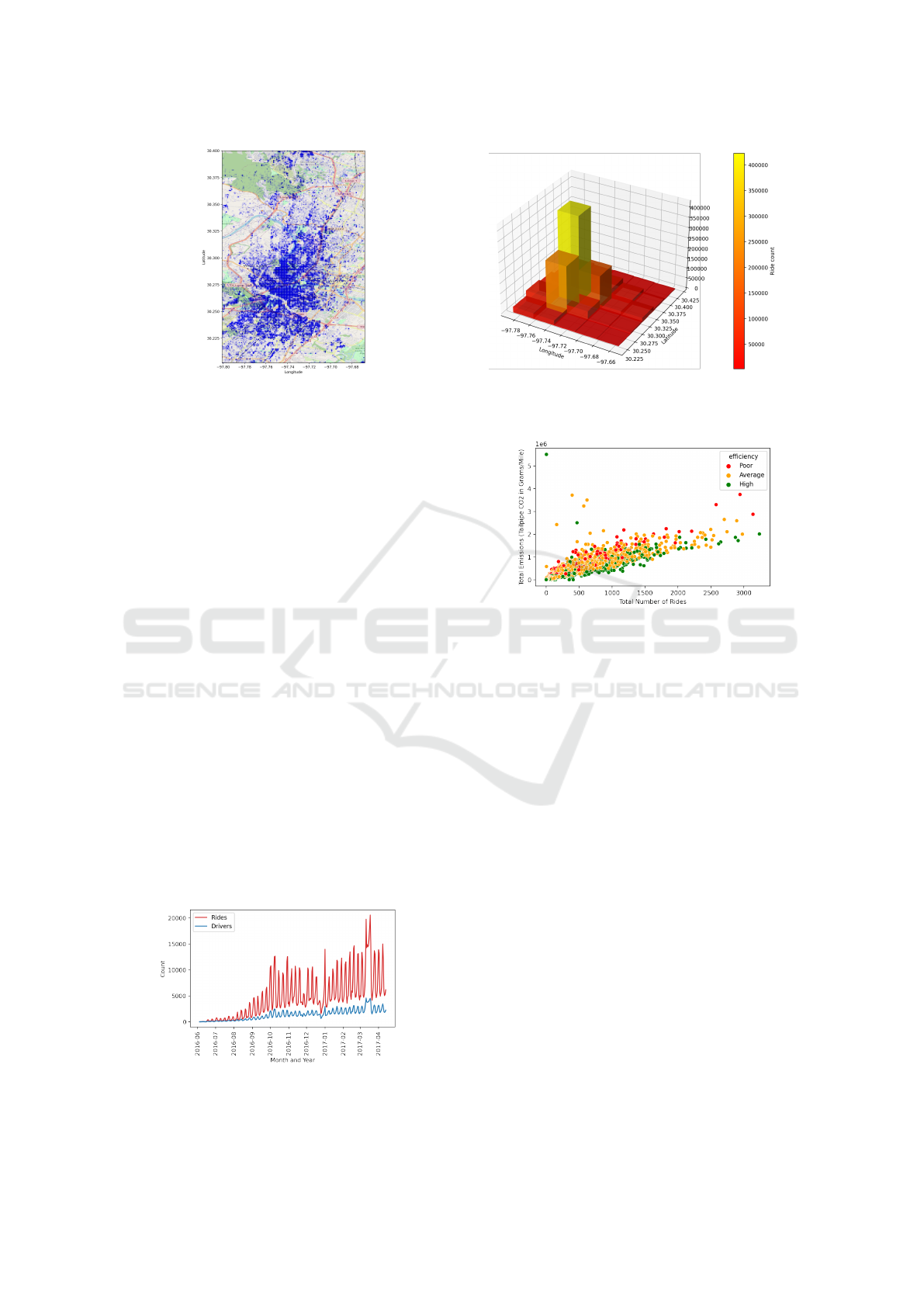
(a) RideAustin pick-up locations in Austin, TX.

(b) RideAustin ride demand distribution.

Figure 1: Pick-up locations and cumulative demand for RideAustin rides (2016-17).

RideAustin Data. RideAustin is a TNC operating

in Austin, Texas, United States, that came into lime-

light after the departure of Uber and Lyft from Austin.

RideAustin published data on over 1.4 million rides,

conducted by over 5000 drivers, over a 11-month pe-

riod (2016-17). Figure 1 describes the pickup loca-

tions and cumulative ride counts for all RideAustin

rides for the given time period. This dataset is a

origin-destination dataset, that has geo-coordinates of

the requested location, start location, end location,

along with corresponding times and distances. Since

riders and drivers are identiﬁed by unique IDs, it is

possible to aggregate by drivers and gain more insight

into their behaviors as well. Figure 2 describes the

daily count of rides and unique drivers. The ﬁgure in-

dicates a consistent weekly oscillation of the counts,

following a trend of much higher supply as well as de-

mand on the weekends compared to weekdays. This

suggests that most riders in Austin used RideAustin

for entertainment and recreational purposes as op-

posed to daily commute to work or school. The sig-

niﬁcant peak near March of 2017 correlates with the

major South by Southwest festival that took place in

Austin. Overall, the number of rides seemed to in-

crease at a greater pace in comparison to the number

of rideshare drivers.

Figure 2: Daily count of rides and drivers through

RideAustin.

Figure 3: Total emissions by vehicle efﬁciency for ﬂeet.

Environmental Protection Agency (EPA) Data.

The U.S. Environmental Protection Agency (EPA)

published a dataset regarding the energy efﬁciencies

of different cars by their model and make. Specif-

ically, the dataset provides a reliable and standard-

ized method of comparing vehicles and their fuel

economies. The dataset included various vehicles’

make and model as well as the associated fuel econ-

omy indicators such as transmission and miles per

gallon (MPG) estimated for “city”, “highway”, and

“combined” conditions. We use this along with the

RideAustin dataset to calculate the emissions pro-

duced by each ride, and consequently for performing

deadheading calculations. We categorize vehicle efﬁ-

ciencies into three categories based on the EPA emis-

sions standards and the underlying data distribution.

The projected EPA CO

emissions standard was 225

g/mi (Agency, 2012), and the calculated 25th empiri-

cal quartile of the EPA dataset is 403.95 g/mi. There-

fore, we take a very conservative approach and cat-

egorize vehicles with less than 330 g/mi CO

emis-

sions per mile under high efﬁciency, greater than 330

g/mi and less than 404 g/mi under average efﬁciency,

and over 404 g/mi under poor efﬁciency. Figure 3

shows how vehicles under the RideAustin ﬂeet with

poor efﬁciency create higher emissions.

VEHITS 2021 - 7th International Conference on Vehicle Technology and Intelligent Transport Systems

194

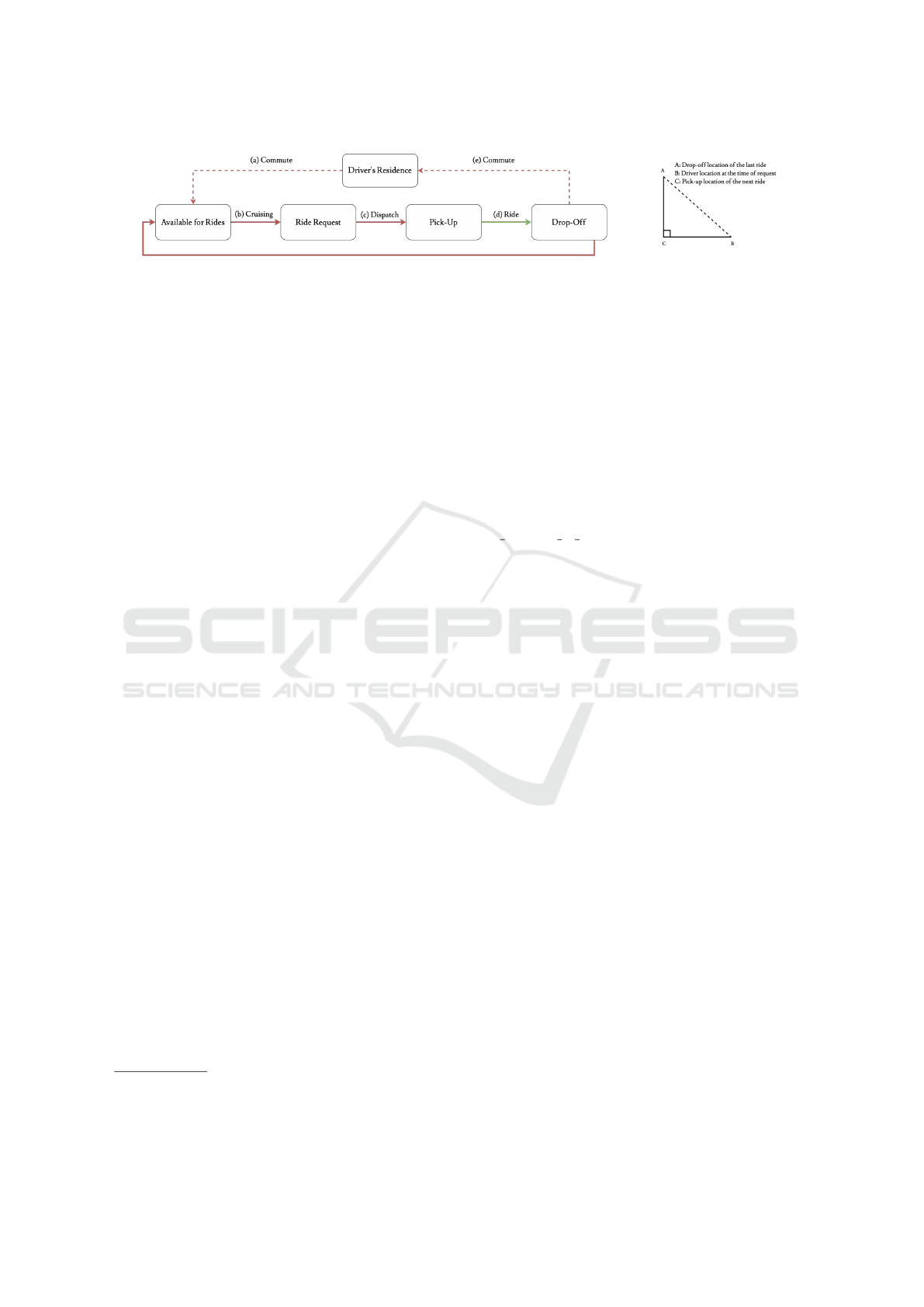
(a) Driving segments in a standard ride-hailing ride.

(b) Inter-ride deadheading.

Figure 4: Calculation of deadheading for a ride-hailing rides.

2.2 Methodology

2.2.1 Overall Deadheading Miles and Emissions

As detailed in Figure 4a, a standard ride-hailing

driver’s mileage and emissions can be divided into

ﬁve segments: (a) commute from a driver’s residence

to the area of service, (b) cruising in search for a ride,

from the passenger pick-up location to the passenger

drop-off location, and (e) commute from the last ride

to the driver’s residence. Segments (b) - (d) recur for

as long as the driver decides to be in service for the

day, all segments but (d) contribute to overall dead-

heading emissions, and segments (b), (c), and (e) con-

tribute to ride deadheading emissions.

To calculate (a) and (e), i.e. deadheading miles

and emissions due to the driver’s daily commute, we

ﬁrst calculate an approximate residential location for

each driver by computing the geometric mean of the

ﬁrst daily coordinates of that driver’s aggregated trips

(Wenzel et al., 2019). We then calculate the haver-

sine distance

between the approximated residential

location and location of the ﬁrst ride starting point,

and between the last ride’s ending point and the ap-

proximated residential location. To account for the

distance over the road network, the origin-destination

straight-line distances for these commutes are multi-

plied by a scaling factor of 1.4, as derived in Wenzel

et al. (2019) from ride-level data, which is annotated

with a GPS-measured distance in addition to origin

and destination coordinates.

To calculate (b), i.e. inter-ride stalling or cruis-

ing, we estimate segment AB in Figure 4b. The

dataset does provide the number of miles driven to

get to a user’s ride request location from the driver’s

current location (BC). However, corrupted dispatch

location data from the dataset resulted in an inabil-

ity to directly compute AB. Therefore, we assume

a 90

◦

angle between segment AC and segment BC.

This value was obtained as a representative of the me-

The haversine formula determines the great-circle distance

between two points on a sphere given their longitudes and

latitudes.

dian between the angle that would produce the largest

amount (180

◦

) and the angle that would produce the

lowest amount (0

◦

) of deadheading. By aggregating

drivers by day, we compute the haversine distance be-

tween the ending location of the previous trip and the

starting location of the following trip to calculate AC.

We then simply compute the Pythagorean distance

and get an estimate for deadheading due to cruising

(AB).

The (c) segment, i.e. the dispatch dis-

tance, is already given in the dataset as the driv-

ing distance to rider parameter.

Finally, we sum (a), (b), (c), and (e) to get the

deadheading miles for each driver for a given day.

This value is multiplied by the emissions efﬁciency

of each driver’s vehicle model and make to estimate

the total deadheading emissions for that driver for that

day. While we identify it necessary to interpolate

these values due to the lack of availability of other in-

formation, we acknowledge that these values may not

be wholly accurate and anticipate that more research

into driver patterns may be beneﬁcial in development

of a more accurate model. Furthermore, we only cal-

culate CO

emissions for simplicity of comparison,

but recognize that other pollutants such as PM, NOx,

NMOG, CO, Formaldehyde, etc. could also serve as

important metrics.

2.2.2 Clustering on Geographical Proximity

The density of ride origins and destinations in Austin

varies greatly with region. For instance, the density

of ride demand around the Airport is much higher

than in any other area (Figure 1b). Therefore, we con-

duct silhouette analysis to determine the optimal k for

k-Means clustering and segment the ride data into k

clusters based on geographical proximity. Silhouette

analysis is a popular graphical technique that allows

for analysis of cluster cohesion and separation, and

is reliable in determining the appropriate number of

clusters for unsupervised learning techniques such as

k-Means (Rousseeuw, 1987).

Ride-hailing Emissions Modeling and Reduction through Ride Demand Prediction

195

2.2.3 Ride Demand Forecasting

We adopt a deep learning approach to forecast hourly

ride demand through spatiotemporal features for each

cluster (or zone). The feature set for each model in-

cludes weather data (humidity, precipitation, heat in-

dex), day of the week, and if that day is a federal hol-

iday. We use a Long Short Term Memory (LSTM)

network to predict the ride demand for the following

hour for each zone. The efﬁcacy of the model is eval-

uated by comparing it against an Extreme Gradient

Boosting (XGBoost) model, which we consider as the

baseline. Each model is described in detail below.

Since our goal is to estimate the reduction in

deadheading emissions through the construction of

this ride demand forecasting model and gauge how it

would generalize in the real world, we choose against

training on several months of data only to evaluate

our results on less than a quarter of the data (as is

prevalent in current literature). Instead, we adopt a

rolling out-of-time evaluation approach to maximize

data coverage and test how our model generalizes

throughout a larger time period. We do this through

running seven sequential iterations of our overarch-

ing model on progressively increasing time windows.

These seven iterations, listed in Table 1, allow for out-

of-time validated ride demand forecasts for a seven-

month period for a given zone.

Table 1: Rolling out-of-time evaluation iterations.

Train Test

Jun ‘16 Jul ‘16

Jun ‘16 - Jul ‘16 Aug ‘16

Jun ‘16 - Aug ‘16 Sep ‘16

Jun ‘16 - Sep ‘16 Oct ‘16

Jun ‘16 - Oct ‘16 Nov ‘16

Jun ‘16 - Nov ‘16 Dec ‘16

Jun ‘16 - Dec ‘16 Aug ‘16

Extreme Gradient Boosting. Gradient boosting

is an algorithm that combines weak base learning

models into a strong learner in an iterative fashion.

Extreme gradient boosting (XGBoost) an improve-

ment on standard gradient boosting, that most notably

uses (i) second-order Taylor expansion, as opposed

to the ﬁrst-order, of the loss function of the base

model; and (ii) L1 and L2 regularization to improve

generalization (Chen and Guestrin, 2016).

Our model is comprised of 1000 sequential deci-

sion trees and a threshold of 50 for early stopping to

prevent overﬁtting. This simple model is considered

as our baseline model for ride demand forecasting.

Long Short-Term Memory. A Long Short-Term

Memory (LSTM) network is a special case of Recur-

rent Neural Networks (RNNs) that is capable of learn-

ing long-term dependencies well enough for practical

purposes. RNNs have a short-term memory - they can

carry information from only the time steps immedi-

ately before. As the time steps increase, the informa-

tion from the earlier time steps is diminished, which

makes RNNs unsuitable for forecasting in cases of

longer time-series sequences.

In contrast, a typical LSTM network constitutes

four layers: a cell state, and three gates - input gate,

forget gate, and output gate - that control the cell state

(Hochreiter and Schmidhuber, 1997). These four lay-

ers iteract and comprise a working model through the

following steps:

1. The forget gate ( f

) decides what information

is to be discarded from the previous cell state,

based on the output of the previous step h

t−1

and

current input X

. The decision is made through

a sigmoid activation function (σ) and the range

is (0, 1), where 0 indicates ‘forget all’, and 1

indicates ‘keep all’. Here, W

represents weights

of the respective neurons and b

represents bias.

= σ(W

t−1

, X

] + b

) (1)

2. In order to decide what new information gets

stored in the cell state, there are two steps that

are later combined. First, the input gate (i

) - a

sigmoid (σ) layer - decides what information is

to be updated. Second, a tanh layer creates C

- a

vector with new candidate values.

= σ(W

t−1

, X

] + b

) (2)

= tanh(W

t−1

, X

] + b

) (3)

tanh =

− e

−x

+ e

−x

(4)

3. The output is also decided by the output gate (o

)

through a two-step process. First, a sigmoid (σ)

layer is run. Second, the cell state (C

) is passed

through tanh and multiplied by the output of the

previous sigmoid layer.

= σ(W

t−1

, X

] + b

) (5)

= o

∗tanh(C

) (6)

Our model is comprised of one LSTM layer with

128 hidden neurons and a corresponding dropout

layer (p = 0.2; where p is the probability of a neuron

being excluded from the network) for regularization.

The model has a look-back interval of 6 time-steps

(i.e. 6 hours), 45 epochs, a batch size of 32, and 10%

of the training data reserved for validation in each

epoch. The chosen loss function is Mean Squared

VEHITS 2021 - 7th International Conference on Vehicle Technology and Intelligent Transport Systems

196

Error (MSE) but Mean Absolute Error (MAE) and

Root Mean Squared Error (RMSE) are also con-

sidered important indicators of model performance.

These are represented below, where n is the number

of observations, Y

is the actual ride demand, and

the predicted ride demand.

MSE =

∑

i=1

−

)

(7)

MAE =

∑

i=1

| Y

−

| (8)

RMSE =

∑

i=1

−

)

(9)

2.2.4 Evaluating Reduction in Deadheading

Emissions

By predicting the location of the next ride, given an

hour-day time bucket, we aim to reduce overall inter-

ride deadheading. We ﬁrst aggregate our set of rides

into buckets for each driver and date. Then, for each

ride and zone, we compute a weighted average of the

distance between the centroid of that zone (obtained

from the earlier k-means clustering) and the current

location of the driver, and the predicted ride demand

for the given hour at that centroid. Through an iter-

ative approach, we found a nearly optimal weighting

of roughly 60% attributed to distance to the centroid

of the driver and 40% to ride demand at that zone.

Given this weighted average, we calculate the op-

timal centroid for each zone as longitude-latitude co-

ordinates. We then calculate the haversine distance

between the location of the last drop-off point and the

centroid (Segment AB, Figure 4b) and the haversine

distance between the location of the centroid and the

next pick-up point (Segment BC, Figure 4b). As ear-

lier mentioned, this value is computed under the as-

sumption that individual drivers are being sent to a

zonal centroid. In other words, after assigning each

driver-ride endpoint to one of 10 zones - computed

by k-means clustering and ride demand forecasting -

we re-route the driver to the centroid of that zone and

stall at that location in preparation for a subsequent

ride. We then aggregate the harversine values to com-

pute an overall prediction for deadheading mileage.

Finally, in a similar manner as in Section 2.2.1,

we utilize the EPA data on vehicular emissions efﬁ-

ciency to compute a value for overall emissions for

each trip by multiplying the calculated deadheading

mileage and the emissions efﬁciency for the vehicle

used for the trip.

3 RESULTS

In this section, we present the results of the afore-

mentioned components of this paper: estimated over-

all deadheading miles and emissions, clusters based

on geographical proximity, efﬁcacy of ride demand

forecasts, and the estimated reduction in deadheading

emissions given our ride demand forecasting model.

3.1 Estimated Deadheading Miles and

Emissions

We estimated that a total of 17,920,612.565 dead-

heading miles and 6014.952 metric tonnes of dead-

heading emissions were produced by the RideAustin

ﬂeet in Austin, Texas from June 2016 - July 2017

(Table 2). These constitute approximately 59% of

all vehicle miles traveled and emissions by the ﬂeet.

Therefore, more empty CO

emissions were produced

than emissions during actual rides. The share of ride

deadheading miles and emissions, which excludes the

deadheading during a driver’s assumed commute to

and back from the service area (as described in 2.2.1),

is slightly lower at 44.4%.

Table 2: Total and deadheading miles and emissions for the

RideAustin ﬂeet (June ‘16 - April ‘17).

Measure VMT (x 10

mi) CO

(tonnes)

Ride DH 1.34 (44%) 4,527.26 (44%)

Overall DH 1.79 (59%) 6,014.95 (59%)

Total 3.03 10,194,499.33

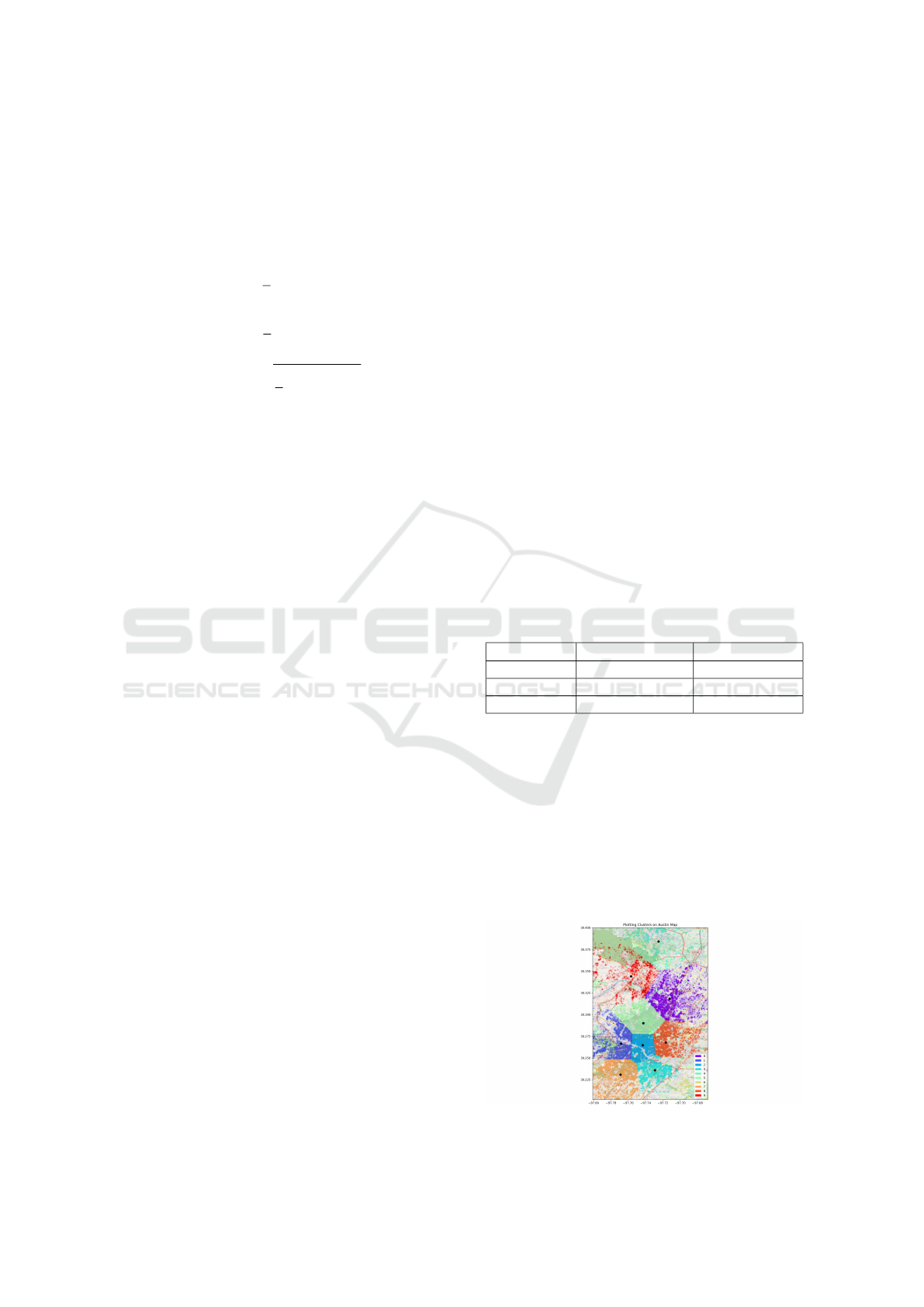
3.2 Geographical Clusters

Through silhouette analysis, we obtained an optimal

value of k = 10 for k-means clustering. As a result of

this clustering, the region covered by the RideAustin

ﬂeet was divided into 10 zones, as depicted in Figure

5. The clusters have different densities - for example,

the Downtown Austin area (represented by Zone 2)

has a much higher density than Zone 5.

Figure 5: Ride demand clusters in Austin, TX.

Ride-hailing Emissions Modeling and Reduction through Ride Demand Prediction

197

3.3 Ride Demand Forecasts

Table 3: Model performance (July ‘16 - Jan ‘17).

Model MAE RMSE

XGBoost (Baseline) 9.36 26.392

LSTM 6.098 18.421

The proposed models were run on the given time in-

tervals and the predictions for the seven-month period

for each zone were combined for each model. The

LSTM-based neural network, which uses spatial fea-

tures in addition to the 6-hour look-back period, far

outperforms the XGBoost model, which we consid-

ered the baseline model for our study (Table 3).

Figure 6 represents the comparison of ride de-

mand forecasts from both models with the actual ride

demand for a randomly selected 3-week time period

(Nov 4, 2016 - Nov 25, 2016). The LSTM model is

able to forecast well even on unnatural peaks during

weekends. Figure 7 speciﬁcally emphasizes the supe-

rior performance of the LSTM model over the base-

line model.

3.4 Estimated Reduction in

Deadheading

If drivers are rerouted based on the hourly ride fore-

casts as estimated by our LSTM model, we estimated

there to be a cumulative 10.624% decrease in total

deadheading miles and emissions in the Austin re-

gion. Figure 8 highlights this difference between the

observed emissions and the revised emissions.

4 DISCUSSION

Our LSTM model outperforms the baseline model by

34.86% and 30.20% in terms of Mean Absolute Er-

ror (MAE) and Root Mean Squared Error (RMSE)

respectively. The model also outperforms a compa-

rable hourly ride demand forecasting model on the

same dataset (Hou et al., 2019) by 15.3% despite a

more robust testing procedure comprised by a much

larger out-of-time validation window. The cumulative

MAE for our model is 6.09 (considering all 10 zones);

this indicates that for any given hour, the model would

predict with an error of around 6 rides on average.

We also estimated the total deadheading emissions

for the recorded period to be 6,014,952 kg CO

. Us-

ing our LSTM model, we estimated there to be a

10.624% reduction in these deadheading emissions.

To give perspective to this number, the amount of

emissions reduced by our proposed model is equiv-

alent to over 661,110 pounds of coal burned, 1,380

barrels of oil consumed, carbon sequestered by 780

acres of US forests in one year, or 130 passenger ve-

hicles driven for one year (EPA, 2020).

We acknowledge that the models and methods

used by us have limitations. Most importantly, while

our estimate of 44.4% ride deadheading is well within

the range of estimates by other researchers (Wenzel

et al., 2019; Cramer and Krueger, 2016; Komanduri

et al., 2018), we do not have a reliable way to validate

our calculations for deadheading miles and emissions.

Speciﬁcally, deadheading commute calculations, i.e.

(a) and (e) in Figure 4a, are based on assumptions and

existing literature, and may differ with each driver’s

speciﬁc behavioral patterns. In addition, the number

of rides through RideAustin progressively increase

over time (Figure 2), especially after August, which

may have affected the forecasting accuracy for earlier

months. Lastly, computational power limitations ren-

dered us unable to optimize the weighted average in

Section 2.2.4 further, but we acknowledge the neces-

sity for improving this ratio.

5 CONCLUSION

In this study, we leveraged data from a ride-hailing

service RideAustin, with over 1.4 million rides and

more than 5000 drivers over an 11-month period, to

perform three tasks: estimate the total deadheading

emissions impact of the RideAustin ﬂeet, build a neu-

ral network to forecast hourly ride demand in it’s ser-

vice area, and estimate the reduction in deadhead-

ing emissions given the aforementioned forecasting

model.

We segmented RideAustin’s service area in

Austin, Texas into 10 zones through a popular un-

supervised learning technique - k-means clustering.

We then built an LSTM-based neural network us-

ing spatiotemporal features to forecast hourly ride

demand for each zone. As a result, we gathered

out-of-time ride demand forecasts for a 7-month pe-

riod for all zones, which allowed us to develop a

model for rerouting drivers based on ride demand. Fi-

nally, we estimated the total reduction in deadhead-

ing emissions given such re-routing. Our LSTM-

based ride demand forecasting model outperforms the

XGBoost-based baseline model by 34.86%, and an-

other state-of-the-art model on the same dataset by

15.3% in terms of Mean Absolute Error (MAE). Fur-

thermore, we estimate a 10.624% reduction in dead-

heading emissions over the 7-month period that the

model was tested on.

We conclude that ride demand forecasting and the

VEHITS 2021 - 7th International Conference on Vehicle Technology and Intelligent Transport Systems

198

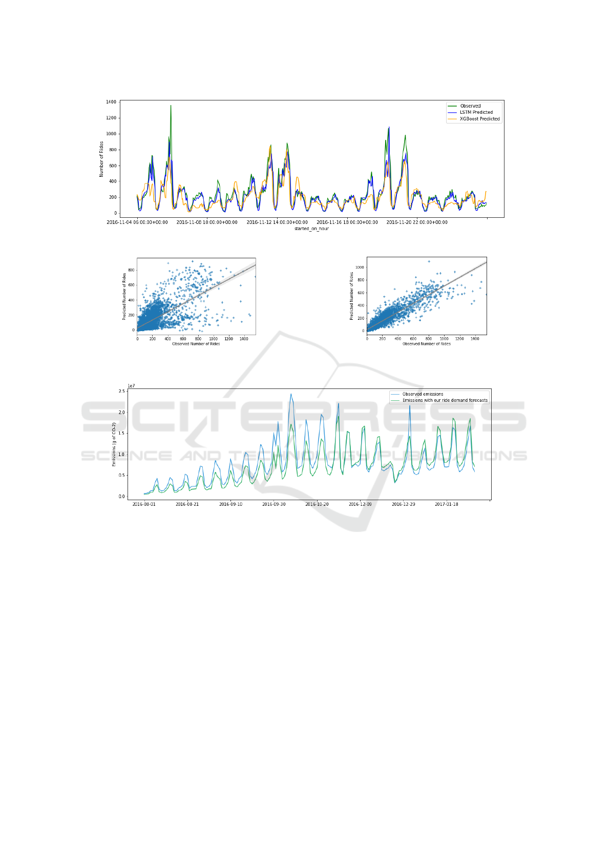
Figure 6: Comparison of ride demand forecasts (Nov ‘2016).

(a) XGBoost

(b) LSTM

Figure 7: Observed vs Predicted ride demand for the following hour.

Figure 8: Emissions reduction through our hourly ride demand forecast.

consequent rerouting of drivers to different geograph-

ical zones in a region has the ability to concretely

reduce deadheading emissions. We strongly believe

that such models could help TNCs reduce their car-

bon footprint in an inexpensive way. In addition to ex-

tending our work through more robust data, potential

future research efforts in this ﬁeld include recording

driver activity in inter-ride periods to better estimate

deadheading and analyzing the impact of facilitating

dedicated parking spaces for ride-hailing drivers on

deadheading emissions. Furthermore, ride-level data

like that collected by Henao et al. (2019) can be

generalized to interpolate mode substitutions for un-

labeled ride data and thus concretely describe patterns

in ridership impacts.

ACKNOWLEDGEMENTS

This study used open data from: RideAustin, The

U.S. EPA, and World Weather Online. This study was

undertaken as part of the ProjectX Machine Learning

Research Competition hosted by the UofT AI organi-

zation at The University of Toronto. We thank Amin

Ghasemazar, University of British Columbia, for his

continued mentorship and feedback. We also thank

the members of the Cornell Data Science project team

for their support.

Ride-hailing Emissions Modeling and Reduction through Ride Demand Prediction

199

REFERENCES

Agency, U. E. P. (2012). Epa and nhtsa set standards to

reduce greenhouse gases and improve fuel economy

for model years 2017–2025 cars and light trucks.

Ahn, K. and Rakha, H. A. (2013). Network-wide impacts of

eco-routing strategies: a large-scale case study. Trans-

portation Research Part D: Transport and Environ-

ment, 25:119–130.

Centobelli, P., Cerchione, R., and Esposito, E. (2017).

Environmental sustainability in the service indus-

try of transportation and logistics service providers:

Systematic literature review and research directions.

Transportation Research Part D: Transport and Envi-

ronment, 53:454–470.

Chen, T. and Guestrin, C. (2016). Xgboost: A scalable

tree boosting system. In Proceedings of the 22nd

acm sigkdd international conf. on knowledge discov-

ery and data mining, pages 785–794.

Clewlow, R. R. and Mishra, G. S. (2017). Disruptive trans-

portation: The adoption, utilization, and impacts of

ride-hailing in the united states.

Cramer, J. and Krueger, A. B. (2016). Disruptive change

in the taxi business: The case of uber. American Eco-

nomic Review, 106(5):177–82.

DPU (2019). Massachusetts rideshare data report. Techni-

cal report, Department of Public Utilities (DPU), Mas-

sachusetts.

EPA, U. (2017). Vehicle fuel economy estimates, 1984-

2017. https://www.kaggle.com/epa/fuel-economy.

Accessed: 2020-10-02.

EPA, U. (2020). Greenhouse gas equivalences calcu-

lator. https://www.epa.gov/energy/greenhouse -gas-

equivalencies-calculator. Accessed: 2020-10-02.

Erhardt, G. D., Roy, S., Cooper, D., Sana, B., Chen, M.,

and Castiglione, J. (2019). Do transportation network

companies decrease or increase congestion? Science

advances, 5(5):eaau2670.

Feigon, S. and Murphy, C. (2016). Shared mobility and the

transformation of public transit. Number Project J-11,

Task 21.

Henao, A. and Marshall, W. E. (2019). The impact of

ride-hailing on vehicle miles traveled. Transportation,

46(6):2173–2194.

Ho, S. C., Szeto, W. Y., Kuo, Y.-H., Leung, J. M., Peter-

ing, M., and Tou, T. W. (2018). A survey of dial-a-

ride problems: Literature review and recent develop-

ments. Transportation Research Part B: Methodolog-

ical, 111:395–421.

Hochreiter, S. and Schmidhuber, J. (1997). Long short-term

memory. Neural computation, 9(8):1735–1780.

Hockstad, L. and Hanel, L. (2018). Inventory of us green-

house gas emissions and sinks. Technical report, En-

vironmental System Science Data Infrastructure for a

Virtual Ecosystem.

Hou, Y., Garikapati, V., Sperling, J., Henao, A., and Young,

S. E. (2019). A deep learning approach for tnc trip

demand prediction considering spatial-temporal fea-

tures. Technical report, National Renewable Energy

Lab.(NREL), Golden, CO (United States).

Jin, G., Cui, Y., Zeng, L., Tang, H., Feng, Y., and Huang, J.

(2020a). Urban ride-hailing demand prediction with

multiple spatio-temporal information fusion network.

Transportation Research Part C: Emerging Technolo-

gies, 117:102665.

Jin, Y., Ye, X., Ye, Q., Wang, T., Chen, J., and Yan, X.

(2020b). Demand forecasting of online car-hailing

with stacking ensemble learning approach and large-

scale datasets. IEEE Access.

Ke, J., Yang, H., Zheng, H., Chen, X., Jia, Y., Gong, P.,

and Ye, J. (2018). Hexagon-based convolutional neu-

ral network for supply-demand forecasting of ride-

sourcing services. IEEE Transactions on Intelligent

Transportation Systems, 20(11):4160–4173.

Komanduri, A., Wafa, Z., Proussaloglou, K., and Jacobs, S.

(2018). Assessing the impact of app-based ride share

systems in an urban context: Findings from austin.

Transportation Research Record, 2672(7):34–46.

Kontou, E., Garikapati, V., and Hou, Y. (2020). Reducing

ridesourcing empty vehicle travel with future travel

demand prediction. Transportation Research Part C:

Emerging Technologies, 121:102826.

RideAustin (2017). Rideaustin data (2017). http://www.

rideaustin.com/.

Rousseeuw, P. J. (1987). Silhouettes: a graphical aid to

the interpretation and validation of cluster analysis.

Journal of computational and applied mathematics,

20:53–65.

Schaller, B. (2018). The new automobility: Lyft, uber and

the future of american cities.

Wang, C., Hou, Y., and Barth, M. (2019). Data-driven

multi-step demand prediction for ride-hailing services

using convolutional neural network. In Science and

Information Conference, pages 11–22. Springer.

Wang, H. and Yang, H. (2019). Ridesourcing systems: A

framework and review. Transportation Research Part

B: Methodological, 129:122–155.

Wenzel, T., Rames, C., Kontou, E., and Henao, A. (2019).

Travel and energy implications of ridesourcing ser-

vice in austin, texas. Transportation Research Part

D: Transport and Environment, 70:18–34.

WorldWeatherOnline (2020). Historical weather api. http:

//www.worldweatheronline.com/developer/api/.

VEHITS 2021 - 7th International Conference on Vehicle Technology and Intelligent Transport Systems

200