Building Indoor Point Cloud Datasets with Object Annotation

for Public Safety

Mazharul Hossain

1 a

, Tianxing Ma

, Thomas Watson

2 b

, Brandon Simmers

, Junaid Ahmed Khan

Eddie Jacobs

and Lan Wang

1 c

Department of Computer Science, University of Memphis, TN, U.S.A.

Department of Electrical and Computer Engineering, University of Memphis, TN, U.S.A.

Department of Electrical and Computer Engineering, Western Washington University, WA, U.S.A.

Keywords:

LiDAR Point Cloud, Indoor Object Detection, Image Dataset, 3D Indoor Map, Public Safety Objects.

Abstract:

An accurate model of building interiors with detailed annotations is critical to protecting the ﬁrst responders’

safety and building occupants during emergency operations. In collaboration with the City of Memphis, we

collected extensive LiDAR and image data for the city’s buildings. We apply machine learning techniques to

detect and classify objects of interest for ﬁrst responders and create a comprehensive 3D indoor space database

with annotated safety-related objects. This paper documents the challenges we encountered in data collection

and processing, and it presents a complete 3D mapping and labeling system for the environments inside and

adjacent to buildings. Moreover, we use a case study to illustrate our process and show preliminary evaluation

results.

1 INTRODUCTION

Fireﬁghter casualties and deaths occur every year due

to the difﬁculties of navigation in smoke-ﬁlled indoor

environments. According to the National Fire Protec-

tion Association, in 2018, 64 ﬁreﬁghters and 3,655

people lost their lives, 15,200 people were injured,

and 25.6 billion dollars were wasted (Fahy and Molis,

2019; Evarts, 2019). The National Institute for Oc-

cupational Safety and Health (NIOSH) provides de-

tailed accounts of ﬁreﬁghter fatalities (CDC/National

Institute for Occupational Safety and Health (NIOSH)

website, 2020). One of the most disheartening threads

in these stories is how close to an exit the ﬁreﬁghters

were found, sometimes less than a mere 10 feet away.

A possible technological solution to this prob-

lem is to use high-quality 3D maps of the interiors

of buildings. These maps can be constructed us-

ing LiDAR. A LiDAR sensor transmits laser pulses,

which are reﬂected by objects in a scene. It mea-

sures the time until each pulse returns, thus determin-

ing the precise distance to the object that reﬂected

the pulse. The sensor builds a dense 3D represen-

https://orcid.org/0000-0002-7470-6140

https://orcid.org/0000-0002-0379-8367

https://orcid.org/0000-0001-7925-7957

tation of the scene by measuring millions of points

distributed across the surfaces of all the objects. Ad-

ditional sensors are used to determine the color of

each point and its overall position in the scene. Maps

formed from these so-called point clouds would then

have hazards and other objects of interest to ﬁrst re-

sponders labeled. The resulting maps could be used

by ﬁreﬁghters or other ﬁrst responders to navigate the

structure and quickly ﬁnd important objects during a

crisis event.

As part of a federally sponsored program, we

have been working with the City of Memphis, Ten-

nessee, USA to use LiDAR and other sensing tech-

nologies along with deep learning algorithms to pro-

duce georeferenced RGB point clouds with per-point

labels. We have encountered many challenges, such

as complex spaces for LiDAR, lack of synchroniza-

tion among different sensor data sources, and uncom-

mon objects not found in existing annotated datasets.

While some of these challenges, e.g., synchronizing

data sources, have been (partly) addressed by existing

research, the majority require new methodologies that

are the focus of our current and future work.

In this paper, we describe our approach to produc-

ing georeferenced 3D building models based on point

cloud and image data for public-safety. Our contri-

butions are as follows. First, we document the chal-

Hossain, M., Ma, T., Watson, T., Simmers, B., Khan, J., Jacobs, E. and Wang, L.

Building Indoor Point Cloud Datasets with Object Annotation for Public Safety.

DOI: 10.5220/0010454400450056

In Proceedings of the 10th International Conference on Smart Cities and Green ICT Systems (SMARTGREENS 2021), pages 45-56

ISBN: 978-989-758-512-8

lenges we encountered in data collection and process-

ing, which may be of interest to researchers in various

areas such as building information modeling, LiDAR

design, machine learning, and public safety. Second,

we describe our complete 3D mapping and labeling

system for building environments including sensors,

data collection processes, and a data processing work-

ﬂow consisting of data fusion, automatic labeling of

hazards and other objects within the data, clustering,

cleaning, stitching, and georeferencing. Third, we use

a case study to illustrate our process and show prelim-

inary evaluation results.

2 RELATED WORK

Generating large-scale 3D datasets for segmentation

is costly and challenging, and not many deep learn-

ing methods can process 3D data directly. For those

reasons, there are few labeled 3D datasets, espe-

cially for indoor environments, at the moment. Below

we describe two public indoor 3D datasets and sev-

eral deep-learning models for object labeling in point

clouds and images.

2.1 Labeled 3D Datasets

ShapeNet Part (Yi et al., 2016) is a subset of the

ShapeNet (Chang et al., 2015) repository which fo-

cuses on ﬁne-grained 3D object segmentation. It con-

tains 31,693 meshes sampled from 16 categories of

the original dataset which include some indoor ob-

jects such as bag, mug, laptop, table, guitar, knife,

lamp, and chair. Each shape class is labeled with two

to ﬁve parts (totaling 50 object parts across the whole

dataset).

Stanford 2D-3D-S (Armeni et al., 2017) is a multi-

modal, large-scale indoor spaces dataset extending

the Stanford 3D Semantic Parsing work (Armeni

et al., 2016). It provides a variety of registered modal-

ities: 2D (RGB), 2.5D (depth maps and surface nor-

mals), and 3D (meshes and point clouds), all with

semantic annotations. The database comprises of

70,496 high-deﬁnition RGB images (1080×1080 res-

olution) along with their corresponding depth maps,

surface normals, meshes, and point clouds with se-

mantic annotations (per-pixel and per-point).

While the above datasets contain a variety of in-

door objects, they do not contain most of the pub-

lic safety related objects needed for our object an-

notation, e.g., ﬁre extinguishers, ﬁre alarms, hazmat,

standpipe connections, and exit signs. Therefore, they

are not immediately useful to our work.

2.2 Object Labeling in Point Clouds

PointNet (Qi et al., 2017a) is a deep neural net-

work that takes raw point clouds as input, and pro-

vides a uniﬁed architecture for both classiﬁcation and

segmentation. The architecture features two subnet-

works: one for classiﬁcation and another for seg-

mentation. The segmentation subnetwork concate-

nates global features with per-point features extracted

by the classiﬁcation network and applies another two

Multi Layer Perceptrons (MLPs) to generate features

and produce output scores for each point. As an im-

provement, the same authors proposed PointNet++

(Qi et al., 2017b) which is able to capture local fea-

tures with increasing context scales by using metric

space distances.

At the beginning of our work, we experimented

with PointNet++ on our point clouds, but found that

many public safety objects, such as ﬁre alarms and

ﬁre sprinklers, are too small for it to segment and clas-

sify correctly. This motivated us to use images to de-

tect and annotate the objects ﬁrst (Section 5.1) and

then transfer the object labels from the images to the

corresponding point clouds to obtain per-point labels

(Section 5.2).

2.3 Object Labeling in Images

Faster R-CNN (Ren et al., 2016) is a deep convolu-

tional neural network (DCNN) model for object de-

tection in the region-based convolutional neural net-

work (R-CNN) machine learning model family. It

produces a class label and a rectangular bounding

box for each detected object. Huang et al. (Huang

et al., 2017) reported that using either Inception

Resnet V2 (Szegedy et al., 2017) or Resnet 101 (He

et al., 2016) as feature extractor with Faster R-CNN

as meta-architecture showed good detection accuracy

with reasonable execution time.

As we needed obtain per-point labels, a rectangu-

lar bounding box was not sufﬁcient. He et al. (He

et al., 2017) extended Faster R-CNN to create Mask

R-CNN which additionally provides a polygon mask

that more tightly bounds an object. It has a bet-

ter overall average precision score than Faster R-

CNN and generates better per-point labels in our point

cloud data. This observation motivated us to adopt

Mask R-CNN in our work.

3 OVERVIEW

We have surveyed seven facilities with 1.86 million

square feet of indoor space that are of interest to pub-

SMARTGREENS 2021 - 10th International Conference on Smart Cities and Green ICT Systems

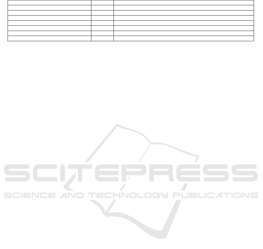
Table 1: List of Buildings.

Name Sqft Use

Pink Palace 170,000 Museum, Theaters, Public Areas, Planetarium, Ofﬁces and Storage

Memphis Central Library 330,000 Library, Public Areas, Storage, Ofﬁces, Retail Store

Hickory Hill Community Center 55,000 Public Area and Indoor Pool

National Civil Rights Museum 100,000 Museum

Liberty Bowl Stadium 1,000,000 Football Stadium with inside and outside areas

FedEx Institute of Technology, U. Memphis 88,675 Reconﬁgurable Facility with Classrooms, Research labs, Ofﬁces, Public Areas

Wilder Tower, U. Memphis 112,544 12-Story Building with Ofﬁces, Computer labs, and Public Areas

lic safety agencies (see Table 1). All the buildings are

located in Memphis. Some of the buildings, e.g., the

Pink Palace, have undergone many renovations which

make it difﬁcult for ﬁrst responders to obtain accurate

drawings. Some buildings, e.g., the Memphis Central

Library, have historical artifacts and important doc-

uments to protect. Others such as the Liberty Bowl

and Wilder Tower have a large number of occupants

to protect in the case of an emergency.

3.1 Challenges

The buildings in our survey represent a wide variety

of structures including a museum, library, nature cen-

ter, store, classroom, ofﬁce, sports stadium, residence,

lab, storage facility, theater, and a planetarium (Ta-

ble 1). They also vary signiﬁcantly in their age, size,

and height. The sizes of the facilities range between

50,000 and 1,000,000 sq ft. Most of the buildings are

between 1 and 4 stories tall, while the Wilder Tower

has 12 ﬂoors in addition to a basement and a pent-

house.

The LiDAR and other equipment we used (Sec-

tion 4.1) are not designed speciﬁcally for an indoor

survey and therefore present several indoor usage

challenges. For instance, it is difﬁcult to scan tight

spaces as the ﬁeld of view of the LiDAR is too small

to generate a complete point cloud. We found the Li-

DAR operator must be at least 1.5 meters away from

the walls, which is hard to achieve in tight spaces. Ad-

ditionally, repeatedly scanning the same space while

turning corners during scanning leads to errors in the

Simultaneous Localization And Mapping (SLAM) al-

gorithm. This occurs when the algorithm cannot rec-

oncile two views of the same scene, so the views

appear randomly superimposed on each other and

the data becomes unusable, requiring the scan to be

restarted. Errors are also likely to occur when open-

ing doors or moving through a doorway, so routes are

planned to minimize these activities. Furthermore,

small errors accumulate as a scan progresses, so scan-

ning must be stopped and restarted, and the pieces

combined later, to avoid the error becoming too large.

Moreover, to avoid stretching our survey over

many days for the larger buildings, we surveyed them

during part of their business hours when there were

occupants in the buildings. This presents an inter-

esting challenge to our data processing algorithms,

i.e., the need to identify and remove humans from the

data. Objects that move during the scan, like humans,

cause further difﬁculty by appearing duplicated be-

cause they are identiﬁed as multiple separate objects.

In addition, we encountered difﬁculties in fusing

LiDAR point clouds and camera images (Section 5.2).

First, we color and assign labels to the points in the

point clouds using the camera images, so they need

to be synchronized precisely. However, the two types

of data are generated by different hardware and soft-

ware, each with its own clock skew. Second, we found

that many points were assigned incorrect labels when

we projected a 2D image to a 3D point cloud. For

example, a window label may be assigned to an ob-

ject behind a window if the object is not labeled in the

image and is visible through the window.

Finally, one challenge associated with object la-

beling is that there are not enough labeled images for

public safety objects because existing datasets focus

on common objects such as chairs and tables (Sec-

tion 5.1). Therefore, identifying ﬁre hydrants, hazmat

signs and other public safety objects of interest re-

quires additional data and training because the state-

of-the-art object detection algorithms have not been

pre-trained on them.

3.2 Approaches

Figure 1 shows our overall process. We use the GVI

LiBackpack 50 which uses a Velodyne VLP-16 Li-

DAR sensor (GVI, 2018) to collect 360 degree Li-

DAR data (Section 4). We modiﬁed the LiBackpack

to mount an Insta360 Pro 2 camera (Insta360 Pro 2

Camera, 2018) that collects 360 degree image data.

The two datasets are collected simultaneously which

facilitates the association of RGB information from

the camera with points from the LiDAR (Section 5.2).

For object detection and segmentation, we use Mask

R-CNN with Inception-ResNet-v2 and ResNet 101 on

our images (Section 5.1). This deep learning network

is trained using the MS COCO dataset (Lin et al.,

2014) and our own labeled images. We then transfer

Building Indoor Point Cloud Datasets with Object Annotation for Public Safety

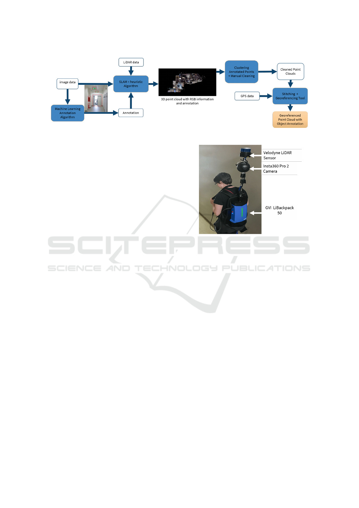
Figure 1: Data Collection and Processing Workﬂow.

the RGB colors and labels from the images to the cor-

responding point clouds (Section 5.2), apply cluster-

ing to the labels in the point clouds, and manually re-

move the falsely labeled objects’ labels (Section 5.3).

Finally, we stitch together all the point clouds for a

building and georeference the ﬁnal point cloud (Sec-

tion 5.4).

4 DATA COLLECTION

In this section, we present our approach to collecting

extensive LiDAR and video data in the surveyed fa-

cilities. We describe our equipment, data types, data

collection workﬂow, and strategies to overcome the

challenges we faced.

4.1 Hardware

The complete list of hardware is below (Figure 2):

• GreenValley International LiBackpack 50

• Velodyne VLP-16 LiDAR

• Surface Pro Tablet

• Insta360 Pro 2 Camera

• Aluminum Tubing

• Reach RS+ RTK GNSS Receiver (GPS receiver)

The LiBackpack’s carbon ﬁber tubing was replaced

with interchangeable sections of aluminum tubing to

allow the sensors to be placed at different heights.

These aluminum pipes connect the LiBackpack to the

bottom of the camera, then the top of the camera to the

Velodyne LiDAR sensor, allowing the sensors to be

worn and operated by one person. This setup rigidly

ﬁxes the camera to the LiDAR, which enables the data

to be properly fused.

The Surface Pro tablet, which is connected to

the LiBackpack via an Ethernet cable, controls the

LiBackpack software and displays the in-progress

scan result for evaluation during scanning. With the

Figure 2: Modiﬁed GVI LiBackpack.

in-progress scan result, it is easy to see whether the

entire area has been scanned or identify problems that

may require rescanning the area.

4.1.1 Video

The video recorded by the camera is stored onto seven

separate SD cards: six SD cards with full resolution

recordings of each of the six lenses, plus one more

SD card with low-resolution replicas, data from the

camera’s internal IMU (inertial measurement unit),

and recording metadata. The video from the six cam-

eras is stitched into a single equirectangular video by

the manufacturer’s proprietary software. This stitched

video has a resolution of 3840 × 1920@30FPS and is

used for all further video processing. Additionally,

this video contains the IMU data, which is used for

time alignment during data fusion.

4.1.2 LiDAR

The backpack stores the raw LiDAR and IMU data

(from its IMU, separate from the camera’s) in the

open-source ROS (Quigley et al., 2009) bag ﬁle for-

mat. The manufacturer’s proprietary on-board soft-

ware performs real-time SLAM processing using this

data to generate a point cloud in PLY format. Because

SMARTGREENS 2021 - 10th International Conference on Smart Cities and Green ICT Systems

the bag ﬁle contains all the data required for SLAM

processing, it can be used to generate an off-board

SLAM result later.

4.2 Data Collection Work Flow

To scan an area, the hardware components are ﬁrst as-

sembled by mounting the LiDAR to the camera, then

mounting the camera to the backpack. Before starting

a scan of a particular area, the operator plans a route

through the space. As discussed in the challenges

above, the operator plans to maximize the distance

from the walls and minimize passage through doors

and crossing previously scanned paths. The scanning

team opens the doors and ensures there are no other

obstacles to the operator, then marks down the area of

the building and the start time of the scan. Once peo-

ple, including the scanning team, are removed from

the space as much as possible, the operator starts the

scan with the tablet and walks through the area, and

stops the scan once ﬁnished. The scanning team then

determines which area should be scanned next and the

process is repeated.

5 DATA PROCESSING

In this section, we present how we process the raw

data collected from buildings to create 3D point

clouds with RGB color and object annotation. First,

we annotate video frames using a machine learning

model. Second, we fuse the labels and RGB data from

video frames with the corresponding point clouds.

Next, we apply a clustering algorithm to identify in-

dividual objects present in the point clouds and man-

ually remove the falsely identiﬁed objects. Finally,

as we scan in parts, we stitch the individual point

clouds into a complete 3D building structure and ap-

ply georeferencing to place it on the world map cor-

rectly. The ﬁnal 3D model can be used in ﬁrst re-

sponse planning, training, and rescue operations, vir-

tual/augmented reality (VR/AR), and many other ap-

plications.

5.1 Annotation

As our point clouds have a resolution of a few cen-

timeters, it is not possible to identify any objects

smaller than that. To address this issue, we instead

apply deep learning to label the objects in the 360-

degree camera images (video frames) and later trans-

fer the labels to the point cloud. We have identiﬁed 30

label classes (Table 2) with high priority, e.g., hazmat,

utility shut-offs (electric, gas, and water), ﬁre alarm

and switch, ﬁre hydrant, standpipe connection, and

ﬁre suppression systems (sprinkler and extinguisher),

from the requirements we collected from ﬁrst respon-

ders and other stakeholders. However, there are two

challenges in annotating the images – lack of good

lighting and cluttered areas. We leverage the im-

provements in object detection algorithms to handle

these challenges. In particular, for the object detec-

tion and segmentation task, we use Mask R-CNN (He

et al., 2017), an extension of Faster R-CNN (Ren

et al., 2016), to create a bounding box and an accu-

rate segmentation mask of each detected object. We

use the Tensorﬂow ofﬁcial model repository for object

detection (Huang et al., 2017), with initial weights

borrowed from their detection model zoo for trans-

fer learning. Figure 3 shows our image annotation

pipeline.

5.1.1 Image Projection

The Insta360 Pro 2 camera has six ﬁsheye lenses.

The video from these lenses is stitched into a 360-

degree equirectangular video with a resolution of

3840 × 1920 with a ﬁeld of view (FOV) of 360 × 180

degrees. We initially reprojected the images into a

cube map, which provides six 960 ×960 images each

with a 90 × 90 degree FOV. The cube map projection

increased the accuracy by avoiding the signiﬁcant dis-

tortion inherent in the equirectangular image. How-

ever, with advancements in our data collection and

manual labeling techniques, we were able to increase

the size of our training dataset, which helped the deep

learning model handle the distortion in equirectangu-

lar projection, leading to similar performance as the

cube map projection. The equiretangular projection

also reduces the processing time signiﬁcantly as there

are six times fewer frames to annotate compared to

the cube map projection.

5.1.2 Manual Annotation

To produce training data for our neural network, we

manually annotated selected frames of video using

LabelMe (Wada, 2016) (Figure 4). Our primary goal

was to annotate at least 100 images from each build-

ing. We have divided the manually annotated images

into training, validation, and test datasets.

5.2 Data Fusion

The hardware has two independent sensors: the video

camera, which records color information, and the

LiDAR, which records depth information. The fu-

sion process transfers RGB and labeled data from the

video frame to the LiDAR point clouds.

Building Indoor Point Cloud Datasets with Object Annotation for Public Safety

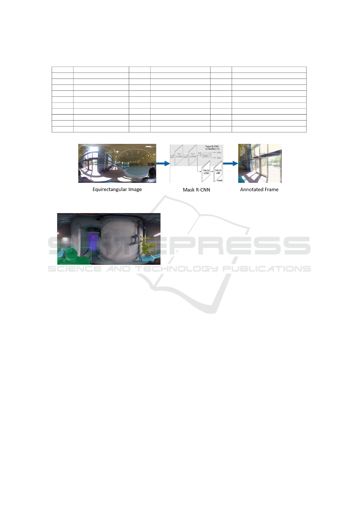
Table 2: List of High Priority Objects.

Priority Label Class Priority Label Class Priority Label Class

5 hazmat 4.2 elevator 3.6 ﬁre door

4.8 utility shut offs - electric 4 ﬁre alarm 3.6 extinguisher

4.8 utility shut offs - gas 4 ﬁre wall 3.6 sign exit

4.8 utility shut offs - water 4 mechanical equipment 3.2 emergency lighting

4.6 building entrance-exit 3.8 sprinkler 3.2 sign stop

4.6 door 3.8 sprinkler cover/escutcheon 3.2 smoke detector

4.6 ﬁre hydrant 3.8 interior structural pillar 3 Automated External Deﬁbrillators

4.4 ﬁre escape access 3.8 standpipe connection 3 Individual First Aid Kit

4.4 roof access 3.8 window 2.4 server equipment

4.4 stairway 3.6 ﬁre alarm switch 2 person

Figure 3: Image Annotation Pipeline.

Figure 4: Manual Annotation Example.

5.2.1 Coloring LiDAR Point Clouds

The fusion process ﬁnds the pixel on the video frame

corresponding to each point in the point cloud and ap-

plies its color to that point. Calculating this corre-

spondence is straightforward because the transforma-

tion between the LiDAR and the camera is known and

ﬁxed. This correspondence is only valid if both sen-

sors capture the depth and pixel information simul-

taneously, thus ensuring they are viewing the same

object. If the system moves too much over the time

between when the depth point and pixel are captured,

the coloring appears blurry and shifted.

We found that reducing this time to 0.05s or less

produced good quality coloring. Unfortunately, we

could not ﬁnd a reliable way of enforcing this. Time

synchronization methods between the LiDAR and

camera were not supported (e.g. hardware trigger

in/out) or would not work in our situation (e.g. GPS

time is not received indoors). However, we can per-

form a coarse synchronization to within 20 seconds

or so by assuming the clocks within the camera and

LiDAR are reasonably accurate. This is enough to

determine which video was being recorded while a

particular LiDAR scan was in progress and provide an

initial guess at what time in that video. Performing the

0.05s alignment is then possible using the IMU data

recorded by both the camera and LiDAR. Because

both IMUs experience the same motion, the time of

maximum correlation between the IMU streams ends

up being the correct alignment around 90% of the

time. The other 10% of the time, the alignment ends

up wildly incorrect, which is obvious during manual

inspection and can then be corrected.

We still had difﬁculties ensuring the clocks were

accurate. The clock in the tablet, used to timestamp

the LiDAR scans, drifted severely, so we had to regu-

larly connect it to the Internet and force a clock syn-

chronization. The clock in the camera could only be

set by connecting it to a phone and hoping a syn-

chronization occurred as it could not be forced. The

camera also frequently forgot the time during battery

changes. We overcame this problem by ensuring the

camera saw the tablet’s clock during each recording,

then correcting the timestamp if it was wrong by read-

ing it from the image of the clock.

5.2.2 Assigning Labels to Points

The annotation process creates label masks for objects

in the camera images. A mask contains all pixels of an

image that are a part of a particular object, along with

the label of that object and the annotation algorithm’s

conﬁdence in the label. Each pixel is labeled as the

SMARTGREENS 2021 - 10th International Conference on Smart Cities and Green ICT Systems

label of the mask that contains it. If multiple masks

contain the pixel, the label with the highest conﬁdence

is used. Some pixels may not be a part of any mask

if they are not part of a recognizable object with a

known label.

In theory, labels can then be applied to the points

in the same way as color. Besides taking the RGB

color of a point’s corresponding pixel, we also take

the label generated from the masks. However, the

implicit mapping of 2D image labels to 3D points

presents some challenges which must be addressed to

improve the ﬁnal labeling quality.

Objects with holes are problematic because the la-

bel masks include the pixels in the object’s holes. For

example, the pixels in a window’s panes are labeled

”window” even though another object might be visi-

ble through them. To address this, we ﬁnd the point

in each mask that is closest to the LiDAR and only

apply the label to points that are not more than 0.5m

farther than that one. We determined experimentally

that objects visible through other objects, like items

visible through windows, almost always exceed this

distance, so incorrect labels for them are effectively

rejected.

Objects in the point cloud are a result of many Li-

DAR captures and camera frames from different times

and positions, so some points of an object may not

be labeled if the corresponding camera frame was far

away or blurry. To ensure such missed points are la-

beled, we ”expand” the point labels to neighboring

points. For each unlabeled point in the ﬁnal labeled

cloud, the closest labeled point within 50mm is lo-

cated. Once all such points have been located, if an

unlabeled point has a close labeled point, its label is

transferred to the unlabeled point. This effectively

ensures all points of an object are labeled, and also

extends the labeled border which helps make smaller

objects more obvious.

5.3 Label Clustering and Manual

Cleaning

We developed an interactive editing tool using

Open3D (Zhou et al., 2018) to enable a user to re-

move falsely labeled objects easily from a 3D point

cloud. It uses DBSCAN (Ester et al., 1996) to cluster

all the points with the same label into individual clus-

ters. This way the users have to deal with only tens

or hundreds of clusters instead of millions of points.

After a user selects and removes the falsely labeled

clusters, the editing tool maps the removed clusters

to the original point clouds and exports the corrected

point clouds. Finally, it merges all the corrected point

clouds (one for each label class) into one point cloud.

5.4 LiDAR Data Stitching and

Georeferencing

For better data quality, we divided each of the build-

ings surveyed into sections and scanned each part sev-

eral times, allowing us to pick the best scan of each

part. To generate a complete building, the selected

parts must all be stitched together. To do this, we used

the “Align by point pair picking” function provided

by the open-source CloudCompare software (Cloud-

Compare v2.10.0, 2019). We choose the larger point

cloud as a reference and use this tool to transform the

smaller point cloud to match the larger one. The tool

calculates the correct transformation once at least 3

pairs of homologous points are picked. We repeat this

process for each piece until we have one point cloud

which contains all parts of the building.

We measure the GPS coordinates of several points

around the building’s exterior using our REACH RS+

device (REACH RS+, 2018). With these points, we

use the alignment tool again to georeference the build-

ing. We chose the WGS 84 / UTM 16N projection

(EPSG:32616) because the point cloud data is already

in meters. The georeferenced data then can be loaded

into ArcGIS Pro (ESRI, 2020) and visualized on a

map.

5.5 VR Visualization

Assessing the quality of the point clouds, including

their color and annotations, is difﬁcult on a computer

monitor. Because the clouds are large and dense 3D

structures, viewing them on a 2D screen shows only

a small part of the story. Rapidly forming an intuitive

understanding of the geometry is difﬁcult. Complex

areas are often mistaken for problematic areas. Iden-

tifying and isolating particular objects requires com-

plex slicing and viewport manipulation.

Since the point clouds are scans of reality, using

virtual reality (VR) to view them seemed natural. To

do this, we use an Oculus Rift S (Oculus VR, 2019)

and the free PointCloudXR (Hertz, 2018) software.

The point clouds are scaled up to real size so that

1 meter in the scan represents 1 meter in VR. This

enables them to be virtually walked through. With

the data presented like it is in reality, examining the

clouds is much easier. With knowledge from watch-

ing the video used for coloring, objects and rooms

can be immediately identiﬁed. Inconsistencies and

glitches stand out and are easily examined.

VR is also a convenient method to effectively

communicate our results. With a minute or so of in-

troduction, stakeholders and other interested users can

examine the clouds themselves and intuitively under-

Building Indoor Point Cloud Datasets with Object Annotation for Public Safety

stand the similarities and differences between the scan

and reality. This lets them get a feel for the advantages

and drawbacks of our methods and the current state of

our work.

Because a good VR experience requires rendering

at very high resolutions and framerates, scans must

usually be downsampled or sliced before they can be

feasibly viewed in VR, which reduces perceived qual-

ity. The software landscape for point clouds in VR

is not mature, and capabilities such as dynamic load-

ing and quality scaling, any form of editing, and most

forms of viewing annotations, are not yet available.

VR is currently just used as a guide to locate and un-

derstand problems so that those areas can be found

and ﬁxed with conventional point cloud editing soft-

ware. Development of more advanced VR software is

one of our future research areas.

5.6 3D Building Maps and Public Safety

A 3D building map with annotations can be viewed on

a computer, tablet, smartphone, or VR headset, serv-

ing a variety of applications in public safety, architec-

ture, computer gaming, and other areas. Below we

elaborate on a few of its usages in public safety.

First, these maps can help ﬁrst responders perform

pre-incident planning more effectively, as they pro-

vide a much more detailed and accurate representa-

tion of indoor space than 2D ﬂoor plans. First respon-

ders and incident commanders can calculate the best

entry/exit points and routes based on the speciﬁc type

and location of an incident before dispatching and on

the way to the incident.

Second, they can be used in 3D simulations to

train ﬁrst responders more safely and less costly. First

responders can put on VR headsets to practice res-

cue operations in their own stations, instead of phys-

ically going into a building under dangerous condi-

tions. Fire, smoke, obstacles, and other digital effects

can be overlaid on the map to simulate different emer-

gency situations.

Third, during a real incident, ﬁrst responders can

use the maps for indoor localization and navigation.

The maps can be viewed through a 3D display in-

tegrated into a ﬁrst responder’s helmet, giving them

sight and information in otherwise dark or smoke

ﬁlled environments. The ﬁrst responders woud also

be outﬁtted with trackers that show their position on

the building map. The 3D display will show them

the safest way out of the building or the fastest way

to reach a speciﬁc location. An incident commander

outside the building can also use map data to locate

responders and guide them inside the building.

Finally, a 3D building map can help building oc-

cupants escape safely in case of an emergency. It can

also help visitors navigate in an unfamiliar building

more easily.

6 CASE STUDY

In this section, we use the Hickory Hill Commu-

nity Center (HHCC) as a case study to show how we

scanned the building, applied a deep learning model

to annotate collected video frames, and fused the ob-

ject labels with the point cloud. We present the per-

formance of the deep learning model on the image

data and the performance of the object labeling on the

point cloud after the data fusion.

6.1 Building Details: Hickory Hill

Community Center (HHCC)

The Hickory Hill Community Center has many com-

plex areas, including an aquatic center with a swim-

ming pool, basketball court with a 2nd ﬂoor walking

track, and a large ﬁtness center, along with many other

indoor facilities, rooms and halls. The large halls and

indoor spaces were easy to scan, but at the same time

the close corridors, small storage rooms, and complex

geometry challenged us. After scanning the whole

building, we re-walked the building and identiﬁed all

the safety-related objects and their locations to create

a complete ground truth. Although it is the small-

est building that we scanned, it still has a variety of

public safety related objects. It contains mechanical

rooms with equipment, hazmat objects, and electrical

shut offs. We identiﬁed other building features such

as the main entry, ﬁre exits, stairways, pillars, doors,

and windows. We also located ﬁre extinguishers, and

a ﬁre hydrant, as well as many ﬁre alarms and ﬁre

alarm switches.

6.2 Annotation

We ﬁrst identiﬁed some images with public-safety ob-

jects from our videos and manually annotated them.

We next trained our Deep Neural Network (DNN)

on these images and used it to annotate all the video

frames. Afterward, we sampled the results to identify

images with false positives and false negatives. Then

we manually annotated these images with the correct

labels, added them to our training dataset (Table 3),

and repeated the process two more times.

We divided the set of manually labeled images

into training, validation, and testing subsets (Table 3).

We report mAP (mean average precision) and mAR

(mean average recall) based on the validation dataset

SMARTGREENS 2021 - 10th International Conference on Smart Cities and Green ICT Systems

(the results of the test dataset were similar to those of

the validation dataset so they are not presented in the

paper). These evaluation metrics are described and

used by Lin et al. (Lin et al., 2014). The mAP is aver-

aged over all 10 IoU thresholds and all 30 categories.

The mAR (AR

) is averaged over all images with a

maximum of 1 detection per image.

6.2.1 Deep Transfer Learning vs. Training DNN

from Scratch

We ﬁrst compared the image annotation performance

with and without transfer learning. As shown in Fig-

ure 5, if we train the neural network from scratch

(blue curve), the mAP increases very slowly and

reaches only 0.15 after 240,000 iterations. If we start

with a model already trained with images from MS

COCO (orange curve), the mAP quickly approaches

0.3 after training with our dataset for only 24,000 it-

erations. Thus, we decided to use the COCO-trained

model, retrain and ﬁne-tune it with our labeled im-

ages, saving computation time and increasing ability.

Figure 5: mAP of Image Annotation with and without

Transfer learning on Validation Dataset (Equirectangular

Projection, Mask R-CNN with ResNet 101).

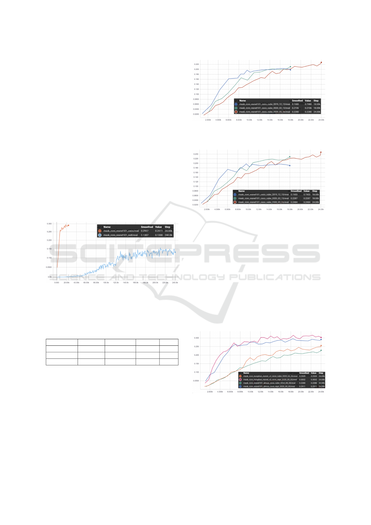
6.2.2 Impact of Adding New Examples

Table 3: Labeled Image Dataset for Training.

Date Training Validation Testing Total

12/13/2019 286 54 0 340

2/13/2020 317 123 125 565

5/5/2020 610 127 128 865

Table 3 shows the change of our training dataset over

time. Figure 6 shows that, as we increased the num-

ber of labeled images in our dataset, the annotation

performance as measured by mAP improved steadily

(the blue, green, and red curves correspond to the

12/13/19, 2/13/20, and 5/5/20 datasets, respectively).

mAR also increased with the size of the training

dataset (Figure 7). We also observed that randomly

adding more images from the same building showed

no increase or even reduced mAP scores (not shown

in the ﬁgures).

Figure 6: mAP of Image Annotation on Different Vali-

dation Datasets (Cube Map Projection, Mask R-CNN with

ResNet 101).

Figure 7: mAR of Image Annotation on Different Vali-

dation Datasets (Cube Map Projection, Mask R-CNN with

ResNet 101).

6.2.3 Impact of Image Projection on Annotation

Accuracy

The panoramas are presented as equirectangular pro-

jection (360 by 180-degree coverage) with a resolu-

tion of 3840× 1920. It is a 2:1 rectangle and straight-

forward to visualize. Initially, we used the equirect-

angular projection, and with each iteration, the gain in

mAP and mAR were negligible. Thus, we decided to

explore the cube map projection which produces six

images of resolution 960× 960, each of which covers

90 × 90 degrees.

Figure 8: mAP - Equirectangular vs Cube Map Projection

Projection on Validation Datasets (Purple is for Mask R-

CNN with Inception ResNet and Blue is for Mask R-CNN

with ResNet 101, both with equirectangular projection. Or-

ange is for Mask R-CNN with Inception ResNet and Green

is for Mask R-CNN with ResNet 101, both with cube map

projection).

Building Indoor Point Cloud Datasets with Object Annotation for Public Safety

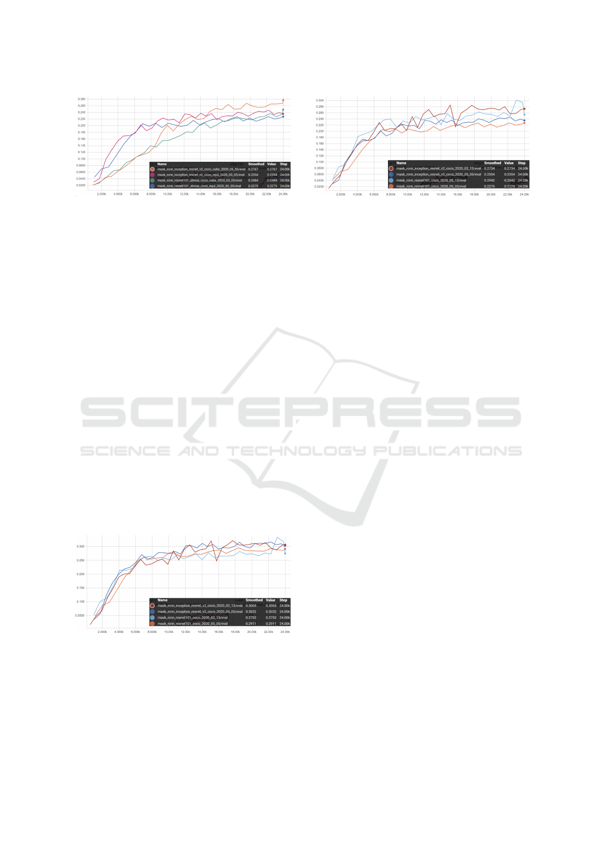
Figure 9: mAP - Equirectangular vs Cube Map Projection

Projection on Validation Datasets (Purple is for Mask R-

CNN with Inception ResNet and Blue is for Mask R-CNN

with ResNet 101, both with equirectangular projection. Or-

ange is for Mask R-CNN with Inception ResNet and Green

is for Mask R-CNN with ResNet 101, both with cube map

projection).

Figure 8 shows that the mAP performance of the

equirectangular projection (purple and blue curves) is

visibly better than that of the cube map projection (or-

ange and green curves), regardless of the DNN. The

mAR performances are much closer for the two pro-

jections and two DNNs as shown in Figure 9. There-

fore, we decided to use the equirectangular projection

for better mAP performance.

6.2.4 Performance Comparison between DNNs

As we were selecting a neural network for our task,

we found that Faster R-CNN was doing slightly bet-

ter than Mask R-CNN. However, as we planned to

transfer our 2D detections to a 3D point cloud, we

chose Mask R-CNN, which provides precise polygon

masks. We then compared two different feature ex-

tractors, Inception-ResNet v2 and ResNet 101, within

Mask R-CNN. Figure 10 and 11 show that Inception-

ResNet v2 and ResNet 101 perform similarly con-

cerning the mAP and mAR metrics.

Figure 10: mAP of Inception-ResNet v2 and ResNet 101 on

Validation Datasets with Equirectangular Projection (Dark

red is for 2/13/20 data and dark blue is for 5/5/20 data, both

with Inception-ResNet v2. Light blue is for 2/13/20 data

and orange is for 5/5/20 data, both with ResNet 101).

Figure 11: mAR of Inception-ResNet v2 and ResNet

101 on Validation Datasets with Equirectangular Projection

(Dark red is for 2/13/20 data and dark blue is for 5/5/20 data,

both with Inception-ResNet v2. Light blue is for 2/13/20

data and orange is for 5/5/20 data, both with ResNet 101).

6.3 Performance Measurement on Point

Cloud

The data fusion process (Section 5.2) transfers the an-

notations in our video frames to the corresponding 3D

point clouds. The resulting 3D point clouds have mul-

tiple error types—some errors carried over from the

image annotation and some errors created during the

data fusion process.

We identiﬁed the individual objects using the DB-

SCAN clustering algorithm. We adjusted DBSCAN

parameter values, such as the maximum distance be-

tween points and the minimum number of points in a

cluster, for different objects to produce a better clus-

tering result. Afterward, we manually removed the

falsely labeled objects using our editing tool.

Table 4 shows the precision and recall for some of

the higher priority objects in the HHCC point cloud

before the manual cleaning. Some types of objects,

e.g., ﬁre extinguishers and ﬁre alarms, have better per-

formance than the others, e.g., building entrance-exits

and elevators. This phenomenon may be due to (a) the

presence of more labeled objects for certain types and

(b) the difﬁculty for the neural network to differen-

tiate building entrance-exits and elevators from other

doors. Note that the table does not include some ob-

jects with zero detection (neither true nor false posi-

tive), e.g., hazmat, as there were very few instances of

them in the training dataset.

7 CONCLUSIONS

We have developed a system to collect and annotate

indoor point clouds with 30 types of public-safety

objects. While the data collection and processing

presented many challenges, we overcame these chal-

lenges by leveraging various existing approaches and

our own methods. Our annotation performance is en-

SMARTGREENS 2021 - 10th International Conference on Smart Cities and Green ICT Systems

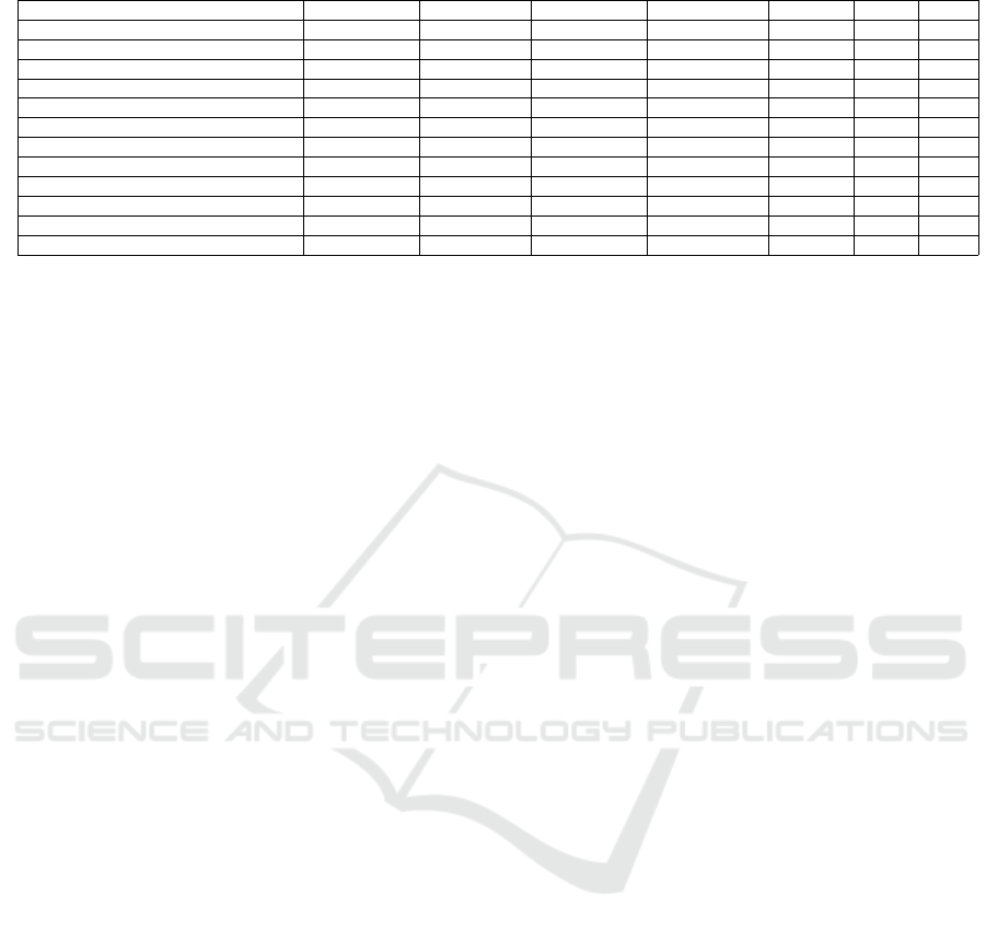
Table 4: Average Precision and Recall of Individual Objects on HHCC Point Cloud.

Name Ground Truth True Positive False Positive False Negative Precision Recall F1

building entrance-exit 14 7 54 7 0.115 0.500 0.187

door 69 69 224 0 0.235 1.000 0.381

elevator 2 2 7 0 0.222 1.000 0.364

ﬁre alarm 64 61 31 3 0.663 0.953 0.782

ﬁre alarm switch 14 7 41 7 0.146 0.500 0.226

ﬁre suppression systems - extinguisher 20 19 6 1 0.760 0.950 0.844

server equipment 2 0 13 2 0.000 0.000 0.000

sign exit 37 37 38 0 0.493 1.000 0.661

smoke detector 4 0 10 4 0.000 0.000 0.000

stairway 1 1 51 0 0.019 1.000 0.038

utility shut offs - electric 49 49 14 0 0.778 1.000 0.875

utility shut offs - water 3 1 6 2 0.143 0.333 0.200

couraging despite our limited training dataset. For

the next step, we plan to improve the annotation per-

formance by addressing the following issues: (a) in-

creasing the number of annotated images for the ob-

jects that are lacking in both our dataset and public

datasets; and (b) improving the recognition accuracy

of small objects such as sprinklers and smoke detec-

tors. We also plan to apply machine learning models

directly to point clouds as a complementary process

to improve the overall accuracy and conﬁdence.

ACKNOWLEDGMENTS

This work was performed under the ﬁnancial assis-

tance award 70NANB18H247 from U.S. Department

of Commerce, National Institute of Standards and

Technology. We are thankful to the City of Memphis,

especially Cynthia Halton, Wendy Harris, Gertrude

Moeller, and Joseph R. Roberts, for assisting us in

collecting data from city buildings, testing our 3D

models, and hosting our data for public access. We

would also like to acknowledge the hard work of our

undergraduate students: Madeline Cychowski, Marg-

eret Homeyer, Abigail Jacobs, and Jonathan Wade,

who helped us scan the buildings and manually an-

notate the image data.

REFERENCES

Armeni, I., Sax, S., Zamir, A. R., and Savarese, S. (2017).

Joint 2d-3d-semantic data for indoor scene under-

standing. arXiv preprint arXiv:1702.01105.

Armeni, I., Sener, O., Zamir, A. R., Jiang, H., Brilakis, I.,

Fischer, M., and Savarese, S. (2016). 3D semantic

parsing of large-scale indoor spaces. In Proceedings

of the IEEE Conference on Computer Vision and Pat-

tern Recognition, pages 1534–1543.

CDC/National Institute for Occupational Safety and Health

(NIOSH) website (2020). Fire ﬁghter fatality investi-

gation and prevention program. https://www.cdc.gov/

niosh/ﬁre/default.html.

Chang, A., Funkhouser, T., Guibas, L., Hanrahan,

P., Huang, Q., Li, Z., Savarese, S., Savva, M.,

Song, S., Su, H., et al. (2015). ShapeNet: An

information-rich 3D model repository. arXiv preprint

arXiv:1512.03012.

CloudCompare v2.10.0 (2019). CloudCompare (version

2.10.0) [GPL software]. http://www.cloudcompare.

org/.

ESRI (2020). ArcGIS Pro (v2.5.0): Next-generation desk-

top GIS. https://www.esri.com/en-us/arcgis/products/

arcgis-pro/overview.

Ester, M., Kriegel, H.-P., Sander, J., Xu, X., et al. (1996).

A density-based algorithm for discovering clusters in

large spatial databases with noise. In KDD, pages

226–231.

Evarts, B. (2019). NFPA report: Fire loss in the

United States during 2018. https://www.nfpa.

org/News-and-Research/Data-research-and-tools/

US-Fire-Problem/Fire-loss-in-the-United-States.

Fahy, R. and Molis, J. (2019). NFPA report: Fire-

ﬁghter fatalities in the US - 2018. https:

//www.nfpa.org//-/media/Files/News-and-Research/

Fire-statistics-and-reports/Emergency-responders/

osFFF.pdf.

GVI (2018). GreenValley International LiBackpack 50.

https://greenvalleyintl.com/hardware/libackpack/.

He, K., Gkioxari, G., Doll

ar, P., and Girshick, R. (2017).

Mask R-CNN. In Proceedings of the IEEE interna-

tional conference on computer vision, pages 2961–

2969.

He, K., Zhang, X., Ren, S., and Sun, J. (2016). Deep resid-

ual learning for image recognition. In 2016 IEEE Con-

ference on Computer Vision and Pattern Recognition

(CVPR), pages 770–778.

Hertz, M. (2018). PointCloud XR virtual reality. http://

www.rslab.se/pointcloud-xr/.

Huang, J., Rathod, V., Sun, C., Zhu, M., Korattikara, A.,

Fathi, A., Fischer, I., Wojna, Z., Song, Y., Guadar-

rama, S., et al. (2017). Speed/accuracy trade-offs for

modern convolutional object detectors. In Proceed-

ings of the IEEE conference on computer vision and

pattern recognition, pages 7310–7311.

Insta360 Pro 2 Camera (2018). Insta360 Pro 2 Camera.

https://www.insta360.com/product/insta360-pro2.

Building Indoor Point Cloud Datasets with Object Annotation for Public Safety

Lin, T.-Y., Maire, M., Belongie, S., Hays, J., Perona, P., Ra-

manan, D., Doll

ar, P., and Zitnick, C. L. (2014). Mi-

crosoft COCO: Common objects in context. In Euro-

pean conference on computer vision, pages 740–755.

Springer.

Oculus VR (2019). Oculus Rift S: PC-powered VR gaming.

https://www.oculus.com/rift-s/.

Qi, C. R., Su, H., Mo, K., and Guibas, L. J. (2017a). Point-

net: Deep learning on point sets for 3d classiﬁcation

and segmentation. In Proceedings of the IEEE con-

ference on computer vision and pattern recognition,

pages 652–660.

Qi, C. R., Yi, L., Su, H., and Guibas, L. J. (2017b). Point-

Net++: Deep hierarchical feature learning on point

sets in a metric space. In Guyon, I., Luxburg, U. V.,

Bengio, S., Wallach, H., Fergus, R., Vishwanathan,

S., and Garnett, R., editors, Advances in Neural Infor-

mation Processing Systems, volume 30. Curran Asso-

ciates, Inc.

Quigley, M., Conley, K., Gerkey, B., Faust, J., Foote, T.,

Leibs, J., Wheeler, R., and Ng, A. Y. (2009). Ros: an

open-source robot operating system. In ICRA work-

shop on open source software, page 5.

REACH RS+ (2018). REACH RS+: Single-band RTK

GNSS receiver with centimeter precision. https://

emlid.com/reachrs/.

Ren, S., He, K., Girshick, R., and Sun, J. (2016). Faster

r-cnn: towards real-time object detection with region

proposal networks. IEEE transactions on pattern

analysis and machine intelligence, 39(6):1137–1149.

Szegedy, C., Ioffe, S., Vanhoucke, V., and Alemi, A. (2017).

Inception-v4, inception-resnet and the impact of resid-

ual connections on learning. In Proceedings of the

AAAI Conference on Artiﬁcial Intelligence.

Wada, K. (2016). LabelMe: Image polygonal annotation

with python. https://github.com/wkentaro/labelme.

Yi, L., Kim, V. G., Ceylan, D., Shen, I.-C., Yan, M., Su, H.,

Lu, C., Huang, Q., Sheffer, A., and Guibas, L. (2016).

A scalable active framework for region annotation in

3d shape collections. ACM Transactions on Graphics

(ToG), 35(6):1–12.

Zhou, Q.-Y., Park, J., and Koltun, V. (2018). Open3D: A

modern library for 3D data processing. arXiv preprint

arXiv:1801.09847.

SMARTGREENS 2021 - 10th International Conference on Smart Cities and Green ICT Systems