PolarNet: Accelerated Deep Open Space Segmentation using Automotive

Radar in Polar Domain

Farzan Erlik Nowruzi

1,2

, Dhanvin Kolhatkar

, Prince Kapoor

,Elnaz Jahani Heravi

Fahed Al Hassanat

1,2

, Robert Laganiere

1,2

, Julien Rebut

and Waqas Malik

School of Electrical Engineering and Computer Sciences, University of Ottawa, Canada

Sensorcortek Inc., Canada

Valeo, France

{julien.rebut, waqas.malik}@valeo.com

Keywords:

Deep Learning, Radar, Open Space Segmentation, Parking, Autonomous Driving, Environment Perception.

Abstract:

Camera and Lidar processing have been revolutionized with the rapid development of deep learning model

architectures. Automotive radar is one of the crucial elements of automated driver assistance and autonomous

driving systems. Radar still relies on traditional signal processing techniques, unlike camera and Lidar based

methods. We believe this is the missing link to achieve the most robust perception system. Identifying drivable

space and occupied space is the ﬁrst step in any autonomous decision making task. Occupancy grid map

representation of the environment is often used for this purpose. In this paper, we propose PolarNet, a deep

neural model to process radar information in polar domain for open space segmentation. We explore various

input-output representations. Our experiments show that PolarNet is a effective way to process radar data that

achieves state-of-the-art performance and processing speeds while maintaining a compact size.

1 INTRODUCTION

Autonomous driving can be approached from various

sensor modalities such as camera, radar, sonar, or li-

dar.

Each sensor provides a piece of valuable informa-

tion. It is shown that the fusion of multiple sensors

is required to cover all of the environmental varia-

tions and achieve fully autonomous driving. Despite

this observation, each individual sensor needs to be

pushed to the edge of its capabilities to reduce the

complexity of the fusion systems.

Radar sensors have been around in the automo-

tive industry for a few decades already. The ﬁrst sys-

tems were mostly used in the premium car segment

for comfort applications, such as Adaptive Cruise

Control (ACC). With the continuous improvement of

radar technology, recent radar sensors are also used in

safety applications, such as Autonomous Emergency

Braking (AEB).

Furthermore, radars are not affected by poor light-

ning and fog, unlike camera and Lidar respectively.

The new versions of radar will signiﬁcantly increase

the resolution of the observations, therefore enabling

an even wider variety of applications.

Ultra-sonic sensors are very similar to radar, with

a focus on close range applications only, such as auto-

mated parking detection. In this paper, we propose a

model to equip radar with the ability to replace ultra-

sonic sensors. In this way, a single sensor can run

in multiple modes to provide better value and reduce

system complexity.

In recent years, deep learning models have

achieved state-of-the-art performance on various

applications (Szegedy et al., 2016)(Ren et al.,

2015)(Redmon and Farhadi, 2018)(Lin et al.,

2017)(Chen et al., 2017)(He et al., 2017)(Qi et al.,

2017). However, these models are rarely used with

automotive radar; traditional signal processing meth-

ods such as Constant False Alarm Rate (CFAR) (Fa-

rina and Studer, 1986)(Minkler and Minkler, 1990)

are commonly used to process radar data. Radar is

an alternative depth sensor that presents a less expen-

sive solution than Lidar at the cost of quality of depth.

Recent advances in radar technology introduced High

Deﬁnition radars that address the issues with the qual-

ity of the depth data. The lack of publicly available

radar datasets could be seen as the primary reason for

the smaller amount of literature in this ﬁeld. This is-

Nowruzi, F., Kolhatkar, D., Kapoor, P., Heravi, E., Al Hassanat, F., Laganiere, R., Rebut, J. and Malik, W.

PolarNet: Accelerated Deep Open Space Segmentation using Automotive Radar in Polar Domain.

DOI: 10.5220/0010434604130420

In Proceedings of the 7th International Conference on Vehicle Technology and Intelligent Transport Systems (VEHITS 2021), pages 413-420

ISBN: 978-989-758-513-5

413

sue is partially addressed by novel datasets with radar

observations (Barnes et al., 2019)(Nowruzi et al.,

2020) that have recently been introduced to enable

the scientiﬁc community to expand the boundaries of

knowledge in this ﬁeld.

In this paper, we introduce a novel deep learning

approach that takes beneﬁt of the polar representation

of the radar observations and performs open space

segmentation in parking lot scenarios. In the past,

these applications relied on traditional signal process-

ing techniques such as Constant False Alarm Rate

(CFAR) that employs hand crafted ﬁlters to detect

points on a potential object. The area can then be seg-

mented into occupied and available spaces based on

these points. We explore using learnable ﬁlters, which

have shown improvements over hand-crafted ones in

many computer vision ﬁelds. Our model relies on a

series of 1D and 2D convolutions that reaches state-

of-the-art segmentation performance in an end-to-end

manner. To address the requirements of the automo-

tive industry, we ensured that the model is compact

and fast to run on embedded platforms. Our contribu-

tions are listed as follows:

1. A deep model, PolarNet, that takes radar frames

in polar coordinate and generates an open-space

segmentation mask in a parking-lot scenario

2. Evaluation of various models and loss functions

for this task

3. Detailed comparison of PolarNet to the state-of-

the-art in terms of performance, speed, and size.

The literature review of deep segmentation model

architectures, along with radar applications, are dis-

cussed in Section 2. A brief description of radar data

can be found in Section 3. The compared model ar-

chitectures are described in Section 4. In Section 5,

various experiments, including the effect on model

performance of using different input data represen-

tations, segmentation models, and loss functions are

evaluated. Furthermore, the computational complex-

ity requirements of each model are discussed in detail.

2 LITERATURE REVIEW

Many research works are proposed to address the

challenge of labeling individual pixels in images for

semantic segmentation. There are two category of

methods in this subject. One uses an encoder-decoder

architecture, and the other uses specialized convolu-

tions to avoid decimating input map size. The com-

plexity of the former approach is highly dependent on

the models used for each component, while the lat-

ter suffers from large memory requirements caused

by maintaining the large feature maps which help in

generating ﬁne segmentation masks.

(Chen et al., 2014) ﬁrst proposed the idea of us-

ing a fully connected conditional random ﬁeld as a

decoder at the end of a deep convolutional model to

extract quality segmentation masks.

Fully Convolutional Network (FCN) (Long et al.,

2015) uses an encoder network, made up of convolu-

tional layers only, to extract intermediate feature maps

of the inputs. By employing skip-connections, up-

sampling, and transposed convolution operations on

the decoder side, an output mask of the desired size is

generated.

Following up with the idea of (Chen et al., 2014),

DeconvNet is introduced in (Noh et al., 2015), and

utilizes a more specialized decoder architecture that

consists of a series of decoupled unpooling and con-

volution layers.

(Badrinarayanan et al., 2017) proposes a similar

architecture to DeconvNet, but with greatly reduced

complexity and compares variations of the FCN, De-

convNet and SegNet models.

The U-Net(Ronneberger et al., 2015) architec-

ture iterates on the FCN model by using deeper de-

coder feature maps and extensive data augmentation.

The U-Net++ (Zhou et al., 2018) architecture is a

more general version of U-Net which signiﬁcantly in-

creases the number and the complexity of the skip

connections between the encoder and the decoder.

(Chen et al., 2018a) pioneered the use of atrous

convolutions for segmentation to avoid subsampling

of the input data, and instead enlarge the ﬁeld of view

of the convolution kernel without using any pooling

layers. Furthermore, multiple parallel atrous con-

volutions are utilized to segment objects at different

scales.

(Zhao et al., 2017) introduced the idea of pyra-

mid pooling to collect global and local information.

(Szegedy et al., 2016) is used with (Chen et al.,

2018a) to build mid-level feature maps. By using par-

allel pooling layers, coarse to ﬁne information is gen-

erated that is later used to extract the ﬁnal segmen-

tation result. (Chen et al., 2018b) merged both cate-

gories of methods by using (Chen et al., 2018a) as the

encoder network and using a small decoder network

to achieve better performance.

To accelerate scene segmentation, (Badino et al.,

2009) considers the space in front of a vehicle free

unless there is a vertical obstacle present. This re-

sulted in the introduction of Stixel as a rectangular

block on the image that identiﬁes vertical surfaces.

Hence, a compressed representation of the environ-

ment is achieved. (Schneider et al., 2016) adds the se-

mantic labels to each stixel. Inspired by these ideas,

VEHITS 2021 - 7th International Conference on Vehicle Technology and Intelligent Transport Systems

414

Stixelnet (Levi et al., 2015) segments an image for

open space using stixel-like rectangular regions. In-

stead of a segmentation model, it relies on a classi-

ﬁcation network that predicts the junction point for

ground and the obstacle. Later, a conditional random

ﬁeld is used to smooth the jittery predictions from the

column-wise network. In this case, each stixel cor-

responds to a speciﬁc angle interval from the camera

point of view. As we explain later, Polar representa-

tion of the radar is well suited for this family of archi-

tectures.

The majority of aforementioned methods rely on

camera based inputs. It is common to use a pre-

trained back-bone to build a new model as training

a completely new architecture is still a challenging

problem. However, in the case of radar input data,

using a pre-trained model from other domains is not a

promising approach. This is due to the fact that there

are various radar representations, and that most radar

processing currently uses traditional techniques (Fa-

rina and Studer, 1986)(Minkler and Minkler, 1990).

Sless et al. (Sless et al., 2019) proposes an encoder-

decoder architecture with a Bird’s Eye View (BEV)

input and a 3-class output: occupied, unoccupied or

unobservable.

Bauer et al. (Bauer et al., 2019) proposed a simi-

lar U-Net architecture for occupancy prediction. They

formulate the classiﬁcation problem as both a three

class problem, as in (Sless et al., 2019), and as a four

class problem. The four-class approach uses an un-

known class to show the certainty of the predictions.

Another issue in the radar domain is the low num-

ber of publicly available datasets that contain some

form of radar data. The NuScenes dataset (Caesar

et al., 2019) is a large-scale dataset developed for au-

tonomous driving. However, the radar data is pro-

vided after processing with traditional models, rather

than providing the raw signal data.

The Oxford Radar RobotCar dataset (Barnes

et al., 2019) is available for scene understanding anal-

ysis. The radar used for data collection offers much

ﬁner resolution and higher range than typical automo-

tive radars. It provides a 360 degree azimuth-range

representation of the received power reﬂection. It is

worth noting that this is 2 dimensional representation.

Raw radar data is not available in this dataset, but the

radar modality provided by the authors is less pro-

cessed than that of the NuScenes dataset. The usage

of specialized hardware uncommon in the automotive

domain due to its physical characteristics is a major

disadvantage for some applications. Most recently,

(Nowruzi et al., 2020) introduced a novel dataset for

open space segmentation in automotive parking sce-

narios. The dataset includes raw radar echos collected

by an automotive grade radar along with the tool chain

to extract various representations. They proposed a

variation of FCN targeted for embedded platform de-

ployment. Their results are evaluated against well-

known deep segmentation models. We rely on this

dataset to benchmark our work.

3 RADAR DATA

To propose a new model, we ﬁrst need to understand

the data that will be used. Raw radar data consists

of a series of echos received from each transmitter-

receiver combination. Each signal consists of multi-

ple chirps and samples. This results in a four dimen-

sional matrix of Samples, Chirps, Transmitters, and

Receivers. It is common that the last two dimensions

are concatenated and stacked as one dimension result-

ing in a three dimensional representation of Samples,

Chirps, and Antennas (SCA). SCA is a raw echo rep-

resentation. Although it includes all the information,

its visualization does not provide much insight into

the data.

To address this, Fast Fourier Transforms (FFT) are

applied along each dimension to achieve the Range,

Doppler, and Azimuth (RDA) representation. The

distance associated with an observation is represented

in the Range dimension, the velocity is represented

in the Doppler dimension, and the angle of arrival of

the signal is represented in the Azimuth dimension.

Note that prior to applying the FFT along the Antenna

dimension, zero-padding is applied along the last di-

mension to achieve the target angle resolution.

RDA = fft



zero pad



fft



fft

(SCA)







(1)

RDA representation is a 3D tensor that, depend-

ing on the view point, shows multiple representations.

For the case of open space segmentation, the most

suitable representation is the RAD view that generates

a polar Range-Azimuth map for each Doppler bin.

Taking log and summing along the Doppler di-

mension results in Range-Azimuth (RA) representa-

tion. RA is a simple 2D BEV of radar data in polar

coordinates.

∑

j=0

log(R

) (2)

RA representations conveys the power responses

received from objects around the vehicle in Polar co-

ordinates. A sample of the RA representation, along

with the annotation, is shown in Figure 1.

PolarNet: Accelerated Deep Open Space Segmentation using Automotive Radar in Polar Domain

415

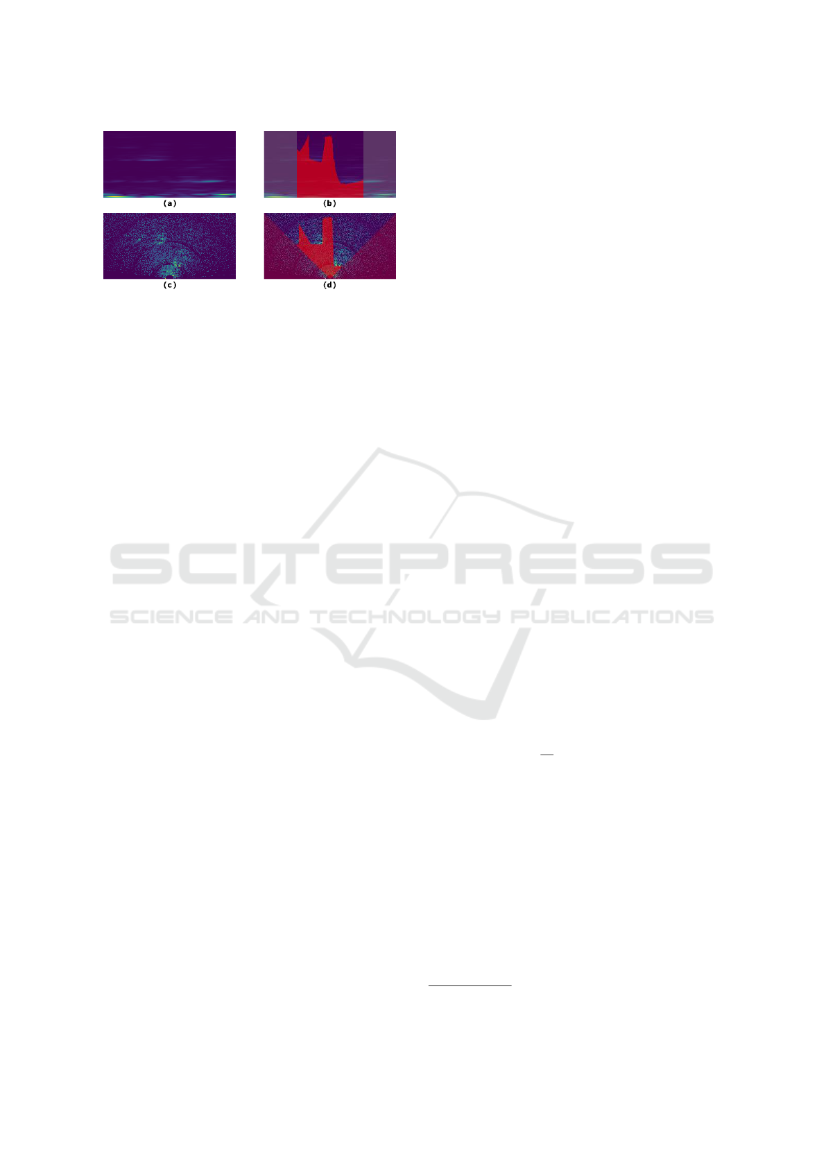
Figure 1: Samples from the dataset. (a) Range-Azimuth

representation. (b) Ground truth annotation on RA. (c) RA

in Cartesian form. (d) Ground-truth projected on Cartesian

map. The angle interval between −45 and +45 is selected

for training.

4 PROPOSED MODEL

PolarNet is a convolutional neural network that is ap-

plied on the RA and RAD representations of radar

observations. In this representation, the ﬁrst dimen-

sion (rows) of the input tensor renders the distance,

while the second dimension (columns) corresponds

to speciﬁc angles. Inspired by StixelNet (Levi et al.,

2015) that uses Stixels, we propose applying one di-

mensional convolutions on each column of the input.

In this way, we apply a ﬁlter on each angle and ef-

fectively try to identify where the open space ends.

Furthermore, by using one-dimensional ﬁlters, we are

reducing the complexity of the network.

PolarNet is an encoder-decoder network with a

smoothing layer at the end of the model. All of the

layers use ReLu as the activation, except for the ﬁnal

two layers that employ Sigmoid activations.

The encoder portion of the model consists of 7

layers. Three of these layers are column-wise con-

volutional ﬁlters that are designed to ﬁnd the location

where the ground meets the ﬁrst obstacle. Another

three layers, positioned after each column-wise lay-

ers, are designed as row-wise convolutions. These

layers are used to pool the information from neigh-

bouring columns, and reduce the size and, conse-

quently, the computational complexity of the model.

Column-wise layers have a stride of 2 along the

columns and row-wise layers use an stride of 2 along

each row. After each column-wise and row-wise

convolution tuple, a batch-normalization (Ioffe and

Szegedy, 2015) and drop-out (Srivastava et al., 2014)

layer is employed. In the last layer of the encoder, we

use a two dimensional 3×3 convolution with a stride

of 1. The output of this layer is concatenated with

the output of layer 6 and is then passed to the decoder

network.

The decoder network consists of a series of con-

volutions and transposed convolutions. Reversing the

order in the encoder, one row-wise transposed con-

volution is applied on the feature map, followed by

a column-wise transposed convolution. The former

layer has a stride of 2 along the columns, while the lat-

ter uses the same stride size along the rows dimension.

The output of this layer is fed to a two dimensional

convolution layer with a kernel size of 5×2. This

layer is responsible for integrating adjacent feature

maps with the goal of reducing jittery artifacts in the

ﬁnal output. We apply the ﬁnal batch-normalization

and drop-out layer. Another column-wise convolu-

tional layer with a larger kernel of 32×1 is used at

this stage, thereby forcing a larger receptive ﬁeld over

the feature map. Radar is capable of observing spaces

behind various objects such as cars. Using this ﬁlter

size, the information from an obstacle is propagated

to those trailing areas. This helps in assigning oppo-

site bits to the ground and non-ground locations; if the

larger receptive ﬁelds are not used, the model will be

confused by the conﬂicting nature of the information

in the input and the mask requirements.

At each layer of the decoder, the depth of the ﬁl-

ter map is consistently reduced. Prior to the ﬁnal

1 × 1 convolution layer that pools all the information

to produce the ﬁnal result, the feature maps are up-

sampled to match the input shape through bilinear up-

sampling. The complete architecture of the proposed

model is shown in Figure 2.

The ﬁnal output contains logits in the range [0,1].

Cells with a value lower than 0.5 is considered as oc-

cupied, while values higher than this threshold are

considered as non-occupied. After this division, a

softmax cross-entropy (SMCE) function is used to ex-

tract the ﬁnal loss value. We use the SMCE

train

loss

function as in (Nowruzi et al., 2020):

SMCE

train

class

∑



∑

−w

× SMCE

+ |w



(3)

where w

represents the trainable weight for class

c, N

is the number of pixels of class c in a particular

groundtruth mask, and SMCE

represents the softmax

cross-entropy loss calculated for a pixel i. As such,

this modiﬁcation of SMCE uses trainable parameters

to weight the SMCE loss on a per-class basis.

A rate of 0.5 is used as drop-out probability. Batch

size is set at 64. RMSProp with initial learning rate

of 0.1 and decay factor of 0.8 at every 3500 steps is

chosen as the optimizer. We use Tensorﬂow

as the

framework to implement and test our model.

www.tensorﬂow.org

VEHITS 2021 - 7th International Conference on Vehicle Technology and Intelligent Transport Systems

416

Figure 2: Detailed architecture of the PolarNet model.

5 EXPERIMENTS

We use the radar dataset of (Nowruzi et al., 2020)

to perform our experiments. This dataset consists

of 3913 frames from 11 sequences with correspond-

ing ground truth. Further, we use their processing

pipeline

to produce RAD and RA representations to

feed as input to our model. Two of these sequences

are left out to make up the test set enabling us to mea-

sure the model’s ability to generalize on previously

unseen scenarios. This ensures the selection of mod-

els that do not overﬁt on the training set.

The annotated points from the Cartesian ground

truth are transformed into the Polar coordinate system

to generate the Polar ground truth information. For

training, RA and RAD tensors are cropped to match

the selected ﬁeld of view. Note that cropping along

columns (angle dimension) equates to reducing the

angular ﬁeld of view in the Cartesian domain.

To benchmark our work we re-use the three deep

learning approaches from (Nowruzi et al., 2020) that

include DeepLabv3+ (Chen et al., 2018b), Fully Con-

volutional Networks (FCN) (Long et al., 2015) and

thier proposal FCN tiny. All three of these segmenta-

tion models use MobileNet-v2 as their back-bone.

DeepLabv2 introduced the idea of replacing con-

volutions with atrous convolutions to increase the ef-

fective ﬁeld of view of a feature extractor without us-

ing the feature extractor’s last 2 pooling layers. The

resulting networks uses much larger feature maps, and

thus has a higher memory cost. The latest version

of this network, DeepLabv3+, uses an atrous spa-

www.sensorcortek.ai/publications/

tial pyramid pooling (ASPP) module, introduced in

DeepLabv2, on the extractor’s output, made up of

atrous convolutions of varying rates and an image

pooling layer in parallel, to help the network detect

objects of varying size. A small decoder, similar to

FCN’s skip architectures, is also used on the ASPP’s

outputs upsampled by a factor of four to reﬁne the

predictions

As in (Nowruzi et al., 2020), we use a complete

version of the DeepLabv3+ architecture with rates of

2, 4 and 6 in the ASPP, in addition to a 1x1 convolu-

tion and an image pooling layer. We remove the last

two pooling layers of MobileNet-v2, and multiply the

convolutions’ rates by 2 after each removed pooling

layer.

The FCN architecture that offers the best compro-

mise between accuracy and speed is the FCN-8’s ar-

chitecture. We use MobileNet-v2 as an encoder and

use two skip architectures as a decoder. Each skip ar-

chitecture works by upsampling its input (either the

encoder’s output, or the previous skip layer’s output)

by a factor of two, then concatenating with the feature

map of matching size taken from the encoder, which

are ﬁrst passed through a 1x1 convolution to reduce

their depth. A 3x3 convolution is applied to the out-

put of the concatenation. As in (Nowruzi et al., 2020),

we use a depth of 32 within the encoder. After two

skip steps, bilinear interpolation is used to resize to

the input size.

(Nowruzi et al., 2020) proposes a smaller version

of MobileNet-v2-FCN-8. It uses a depth multiplier of

0.25 in the encoder, and a set depth of 8 in the decoder

(25% of the full FCN’s decoder depth).

As in most segmentation literature, we use Mean

PolarNet: Accelerated Deep Open Space Segmentation using Automotive Radar in Polar Domain

417

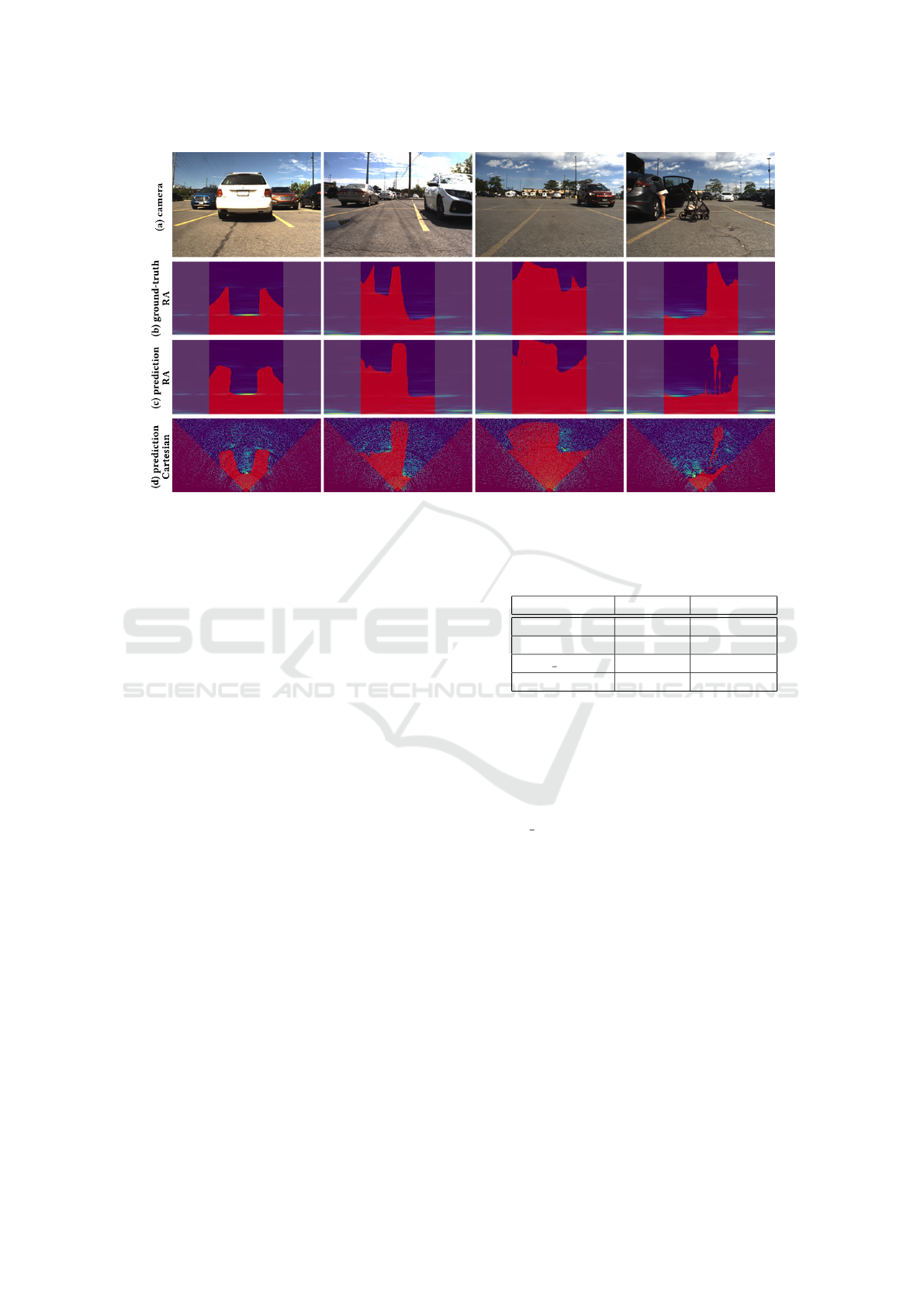
Figure 3: Sample results of PolarNet. (a) camera image. (b) ground-truth in polar coordinates. (c) segmentation result. (b)

segementation result shown in Cartesian coordinates.

Intersection-over-Union (Mean-IoU) as the evalua-

tion metric. This metric is calculated as the mean of

the IoU’s for each class in the dataset. Sample re-

sults of the proposed model in both Cartesian and po-

lar forms, along with the matching ground truths and

camera images, are shown in Figure 3.

Our experiments section is divided into three.

First, we compare the effect of various input represen-

tations on the performance of the model. Second, we

evaluate the effectiveness of various loss functions.

Finally, we compare the computational performance

and size of our model against the state-of-the-art on

multiple platforms.

5.1 Input Representation

PolarNet is designed to be applied on polar repre-

sentations; these include the Range-Azimuth-Doppler

(RAD) and the Range-Azimuth (RA) representations.

RAD is a tensor of size 128 × 128 × 64. Each range

bin is approximately 11.17cm with a maximum range

of 15m that covers an angle interval of −45 to +45

degrees. The third dimension represents the Doppler

bins that cover a velocity range between −37.3 kmph

and +37.3kmph. The RA representation is calculated

from the RAD representation by selecting the maxi-

mum values along the Doppler bins for each Range-

Azimuth index.

Table 1 shows the comparative results of PolarNet

against the state-of-the-art.

Our proposed PolarNet model is the best per-

former with RA inputs. While using RAD results

Table 1: Mean-IoU comparison of models with different

inputs.

Model RA input RAD input

FCN 83.98 85.16

DeepLabV3+ 83.01 83.58

FCN tiny 84.18 83.14

PolarNet 84.20 83.79

in a performance reduction for PolarNet, it still takes

second place behind the much larger FCN model as

shown in Table 3. From the experiments, we observe

that the larger models have an easier time manag-

ing RAD inputs that contain 64 times more informa-

tion than RA inputs. Inversely, smaller models such

as FCN tiny and PolarNet have a harder time han-

dling this huge dimensionality increase. As we see in

the next sections, the small reduction in performance

comes with a larger advantage in the computational

complexity of the system.

5.2 Loss Functions

We compare three loss functions for this task:

trainable softmax cross-entropy loss, softmax cross-

entropy and Lovasz loss (Berman et al., 2017).

SMCE is commonly used as an extension of the

typical classiﬁcation task to the segmentation task;

the loss is calculated independently on a per-pixel ba-

sis and then averaged over the entire image. To aid

in training using SMCE, it is better to use a weight-

ing parameter to reduce effect of any imbalance on

VEHITS 2021 - 7th International Conference on Vehicle Technology and Intelligent Transport Systems

418

data. However, tuning this extra hyper-parameter can

be cumbersome. Another interesting function to con-

sider is the Lovasz loss. It enables optimization of

the mean IoU metric directly, thereby showing a di-

rect link between the main metric for segmentation

and the optimization of the loss function. We com-

pare these two functions with the loss function used

in our previous experiments: SMCE

train

PolarNet architecture is used with RA inputs to

evaluated mentioned loss functions. Results are re-

ported in Table 2.

Table 2: Mean-IoU for PolarNet with RA input and polar

labels using different loss functions.

Loss Function Mean-IoU

SMCE

train

84.20

SMCE 82.02

Lovasz 82.85

SMCE

train

achieved the best results in this experi-

ment. Weighting parameter learning in SMCE

train

re-

sults in its better performance in comparison to the

original SMCE and Lovasz that both lack the weight-

ing functionality. This has shown to be the key differ-

entiator in the performance of the models.

5.3 Complexity Analysis

Our ﬁnal analysis concerns the computational com-

plexity and the speed of our model architectures. It is

crucial for the models to target embedded deployment

and real-time performance on such systems. The de-

tails of our experiments for the proposed model archi-

tectures are shown in Table 3.

DeepLabV3+ is the largest model with slowest

performance in both RA and RAD input cases. Sur-

prisingly, the segmentation performance of this model

is also inferior to the other models. FCN is 90% of

the size of DeepLabV3+ and almost 10% faster on a

Geforce RTX2080 TI GPU. However, on a Core i9-

9900K CPU, it is almost twice as fast. This trend can

be observed on the Jetson TX2 as well.

FCN is still a large model when considering

a Radar on Chip (RoC) product. PolarNet and

FCN tiny address this challenge. PolarNet is one ﬁfth

of the size of DeepLabV3+. It runs more than 2.5

times faster on Jetson TX2 while providing the best

mean-IoU on RA and second best on RAD.

The main advantage of FCN tiny against Polar-

Net is its smaller parameter space. FCN tiny perfoms

faster on the Jetson’s CPU than PolarNet, but Polar-

Net outperforms FCN tiny on the Jetson TX2 GPU.

This is similar to the behaviour of DeepLabv3+ and

FCN. In case of PolarNet, this can be attributed to the

fact that PolarNet uses larger convolution kernels that

are faster to calculate on GPU than on CPU because

of their vectorized computation.

6 CONCLUSION

In this paper, we proposed a novel deep model, Po-

larNet, to segment open spaces in parking scenarios

using automotive radar. Our model takes beneﬁt of

vectorized GPU operations and outperforms the state-

of-the-art in terms of speed.

Furthermore, PolarNet provides the state-of-the-

art performance using Range-Azimuth as its input

modality. These characteristics of the model make it

the perfect candidate for RoC integration scenarios.

We have proposed a single frame model. To fur-

ther increase the performance of this model, tempo-

ral ﬁltering methods could be used: aggregating pre-

dictions at various timesteps would reduce the noise

in the segmentation mask. However, this will result

in more parameters and larger computational require-

ments that needs to be addressed prudently.

REFERENCES

Badino, H., Franke, U., and Pfeiffer, D. (2009). The stixel

world-a compact medium level representation of the

3d-world.

Badrinarayanan, V., Kendall, A., and Cipolla, R. (2017).

Segnet: A deep convolutional encoder-decoder ar-

chitecture for image segmentation. IEEE Transac-

tions on Pattern Analysis and Machine Intelligence,

39(12):2481–2495.

Barnes, D., Gadd, M., Murcutt, P., Newman, P., and Pos-

ner, I. (2019). The oxford radar robotcar dataset: A

radar extension to the oxford robotcar dataset. arXiv

preprint arXiv: 1909.01300.

Bauer, D., Kuhnert, L., and Eckstein, L. (2019). Deep, spa-

tially coherent inverse sensor models with uncertainty

incorporation using the evidential framework. 2019

IEEE Intelligent Vehicles Symposium (IV).

Berman, M., Triki, A. R., and Blaschko, M. B. (2017). The

lov

asz-softmax loss: A tractable surrogate for the op-

timization of the intersection-over-union measure in

neural networks.

Caesar, H., Bankiti, V., Lang, A. H., Vora, S., Li-

ong, V. E., Xu, Q., Krishnan, A., Pan, Y., Baldan,

G., and Beijbom, O. (2019). nuscenes: A multi-

modal dataset for autonomous driving. arXiv preprint

arXiv:1903.11027.

Chen, L.-C., Papandreou, G., Kokkinos, I., Murphy, K., and

Yuille, A. L. (2014). Semantic image segmentation

with deep convolutional nets and fully connected crfs.

arXiv preprint arXiv:1412.7062.

PolarNet: Accelerated Deep Open Space Segmentation using Automotive Radar in Polar Domain

419

Table 3: Computational complexity comparison for the tested methods.

Input RA RAD

Model PolarNet FCN tiny FCN DeepLabv3+ PolarNet FCN tiny FCN DeepLabv3+

GPU (fps) 575.01 324.50 300.75 275.15 364.89 249.79 224.56 199.83

CPU (fps) 271.39 267.58 118.56 61.91 208.14 189.12 133.78 61.93

TX2 GPU (fps) 54.65 31.91 29.18 22.39 48.18 28.87 28.91 21.46

TX2 CPU (fps) 25.90 41.62 22.20 10.46 17.97 36.86 19.68 10.09

# parameters 562,472 210,279 2,933,449 3,223,865 598,758 214,817 2,951,593 3,242,009

Memory cost 29.85 Mb 16.02 Mb 59.64 Mb 134.86 Mb 39.79 Mb 23.04 Mb 70.81 Mb 143.74 Mb

Chen, L.-C., Papandreou, G., Kokkinos, I., Murphy, K.,

and Yuille, A. L. (2018a). Deeplab: Semantic im-

age segmentation with deep convolutional nets, atrous

convolution, and fully connected crfs. IEEE Trans-

actions on Pattern Analysis and Machine Intelligence,

40(4):834–848.

Chen, L.-C., Papandreou, G., Schroff, F., and Adam, H.

(2017). Rethinking atrous convolution for semantic

image segmentation.

Chen, L.-C., Zhu, Y., Papandreou, G., Schroff, F., and

Adam, H. (2018b). Encoder-decoder with atrous sep-

arable convolution for semantic image segmentation.

Lecture Notes in Computer Science, page 833–851.

Farina, A. and Studer, F. A. (1986). A review of cfar detec-

tion techniques in radar systems. Microwave Journal,

29:115.

He, K., Gkioxari, G., Doll

ar, P., and Girshick, R. (2017).

Mask r-cnn.

Ioffe, S. and Szegedy, C. (2015). Batch normalization: Ac-

celerating deep network training by reducing internal

covariate shift. arXiv preprint arXiv:1502.03167.

Levi, D., Garnett, N., Fetaya, E., and Herzlyia, I. (2015).

Stixelnet: A deep convolutional network for obstacle

detection and road segmentation.

Lin, T.-Y., Goyal, P., Girshick, R., He, K., and Doll

ar, P.

(2017). Focal loss for dense object detection.

Long, J., Shelhamer, E., and Darrell, T. (2015). Fully con-

volutional networks for semantic segmentation.

Minkler, G. and Minkler, J. (1990). Cfar: the principles of

automatic radar detection in clutter. NASA STI/Recon

Technical Report A, 90.

Noh, H., Hong, S., and Han, B. (2015). Learning deconvo-

lution network for semantic segmentation.

Nowruzi, F. E., Kolhatkar, D., Kapoor, P., Heravi, E. J., La-

ganiere, R., Rebut, J., and Malik, W. (2020). Deep

open space segmentation using automotive radar.

Qi, C. R., Yi, L., Su, H., and Guibas, L. J. (2017). Point-

net++: Deep hierarchical feature learning on point sets

in a metric space.

Redmon, J. and Farhadi, A. (2018). Yolov3: An incremental

improvement.

Ren, S., He, K., Girshick, R., and Sun, J. (2015). Faster

r-cnn: Towards real-time object detection with region

proposal networks.

Ronneberger, O., Fischer, P., and Brox, T. (2015). U-net:

Convolutional networks for biomedical image seg-

mentation. Medical Image Computing and Computer-

Assisted Intervention – MICCAI 2015, page 234–241.

Schneider, L., Cordts, M., Rehfeld, T., Pfeiffer, D., En-

zweiler, M., Franke, U., Pollefeys, M., and Roth, S.

(2016). Semantic stixels: Depth is not enough.

Sless, L., Cohen, G., Shlomo, B. E., and Oron, S. (2019).

Road scene understanding by occupancy grid learning

from sparse radar clusters using semantic segmenta-

tion.

Srivastava, N., Hinton, G., Krizhevsky, A., Sutskever, I.,

and Salakhutdinov, R. (2014). Dropout: a simple way

to prevent neural networks from overﬁtting. The jour-

nal of machine learning research, 15(1):1929–1958.

Szegedy, C., Ioffe, S., Vanhoucke, V., and Alemi, A. (2016).

Inception-v4, inception-resnet and the impact of resid-

ual connections on learning.

Zhao, H., Shi, J., Qi, X., Wang, X., and Jia, J. (2017). Pyra-

mid scene parsing network. 2017 IEEE Conference on

Computer Vision and Pattern Recognition (CVPR).

Zhou, Z., Siddiquee, M. M. R., Tajbakhsh, N., and Liang,

J. (2018). Unet++: A nested u-net architecture for

medical image segmentation.

VEHITS 2021 - 7th International Conference on Vehicle Technology and Intelligent Transport Systems

420