Virtual Outcrops Building in Extreme Logistic Conditions for Data

Collection, Geological Mapping, and Teaching: The Santorini’s

Caldera Case Study, Greece

Fabio Luca Bonali

1,2 a

, Luca Fallati

, Varvara Antoniou

, Kyriaki Drymoni

Federico Pasquaré Mariotto

, Noemi Corti

, Alessandro Tibaldi

1,2 g

, Agust Gudmundsson

and Paraskevi Nomikou

Department of Earth and Environmental Sciences, University of Milano-Bicocca, Piazza della Scienza 4,

Ed. U04, 20126, Milan, Italy

CRUST- Interuniversity Center for 3D Seismotectonics with Territorial Applications, Italy

Department of Geology and Geoenvironment, National and Kapodistrian University of Athens,

Panepistimioupoli Zografou, 15784 Athens, Greece

Department of Earth Sciences, Queen's Building, Royal Holloway University of London, Egham, Surrey TW20 0EX, U.K.

Department of Human and Innovation Sciences, Insubria University, Via S. Abbondio 12, 22100 Como, Italy

Kyriaki.Drymoni.2015@live.rhul.ac.uk, n.corti3@campus.unimib.it, pas.mariotto@uninsubria.it,

Agust.Gudmundsson@rhul.ac.uk

Keywords: Virtual Outcrops, Photogrammetry, Structure from Motion, Santorini Volcano, Caldera, Dykes.

Abstract: In the present work, we test the application of boat-camera-based photogrammetry as a tool for Virtual

Outcrops (VOs) building on geological mapping and data collection. We used a 20 MPX camera run by an

operator who collected pictures almost continuously, keeping the camera parallel to the ground and opposite

to the target during a boat survey. Our selected target was the northern part of Santorini’s caldera wall, a

structure of great geological interest. A total of 887 pictures were collected along a 5.5-km-long section along

an almost vertical caldera outcrop. The survey was performed at a constant boat speed of about 4 m/s and a

coastal approaching range of 35.8 to 296.5m. Using the Structure from Motion technique we: i) produced a

successful and high-resolution 3D model of the studied area, ii) designed high-resolution VOs for two selected

caldera sections, iii) investigated the regional geology, iv) collected qualitative and quantitative structural data

along the vertical caldera cliff, and v) provided a new VO building approach in extreme logistic conditions.

1 INTRODUCTION

Field studies and data collection are vital components

for geological mapping and for understanding the

active processes on Earth, with particular regard to

shallow magmatic ones (e.g. Tibaldi and Bonali,

2017; Gudmundsson, 2020). Field studies can be

https://orcid.org/0000-0003-3256-0793

https://orcid.org/0000-0002-5816-6316

https://orcid.org/0000-0002-5099-0351

https://orcid.org/0000-0001-7262-8719

https://orcid.org/0000-0003-2157-8760

https://orcid.org/0000-0002-0798-6429

https://orcid.org/0000-0003-2871-8009

https://orcid.org/0000-0001-8842-9730

challenging, due to particular field-related conditions,

that cause limited outcrop accessibility and result in

poor data collection.

Thus, mapping and data collection on Unmanned

Aerial Vehicles (UAVs)-based photogrammetry-

derived Digital Surface Models (DSMs),

Orthomosaics and Virtual Outcrops (VOs), have

become standard practice, especially in volcanic areas

Bonali, F., Fallati, L., Antoniou, V., Drymoni, K., Mariotto, F., Corti, N., Tibaldi, A., Gudmundsson, A. and Nomikou, P.

Virtual Outcrops Building in Extreme Logistic Conditions for Data Collection, Geological Mapping, and Teaching: The Santorini’s Caldera Case Study, Greece.

DOI: 10.5220/0010419300670074

In Proceedings of the 7th Inter national Conference on Geographical Information Systems Theory, Applications and Management (GISTAM 2021), pages 67-74

ISBN: 978-989-758-503-6

(e.g. Bonali et al., 2020; Tibaldi et al., 2020). VOs are

also known as digital outcrop models, which are a

digital 3D representation of the outcrop surface (e.g

Xu et al., 1999). By contrast, static camera-based

outcomes are rare and restricted to narrow-sized

surveys on small field-scale geological features (e.g.

Scott et al., 2020).

In this paper, we test the use of camera-based

photogrammetry for reconstructing the northern part

of Santorini’s caldera wall (Fig. 1) for subsequent

geological studies. The wall represents an outstanding

vertical outcrop of layered deposits dissected by a

well-exposed local dyke swarm (Figs. 2a-b). It is

characterized by extreme logistic conditions

preventing efficient field and UAV surveys due to its

steepness and elevation (max height of 330 m a.s.l.).

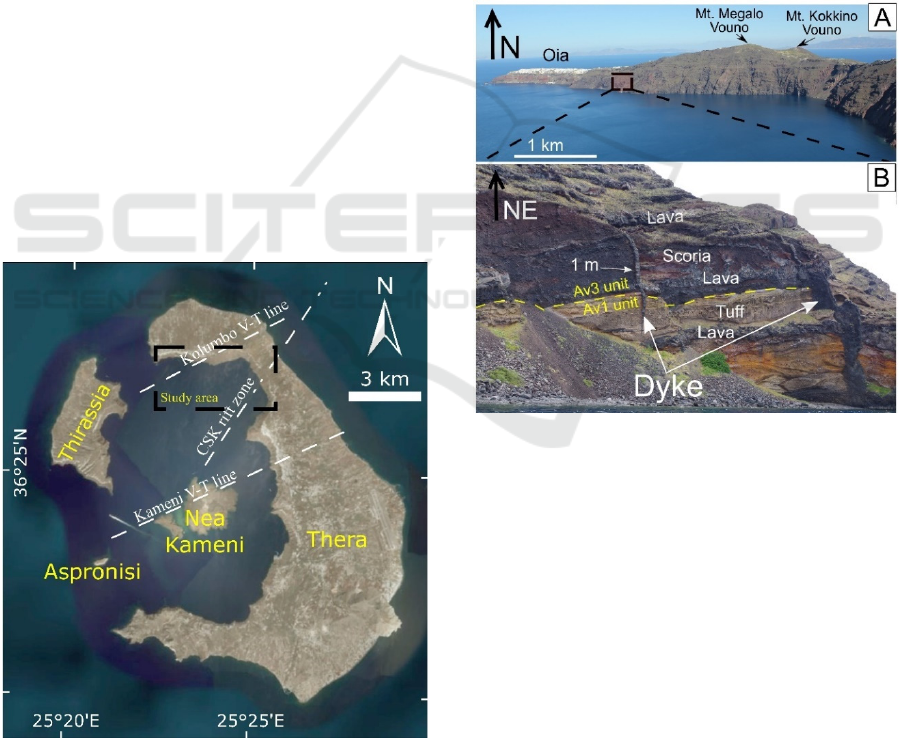
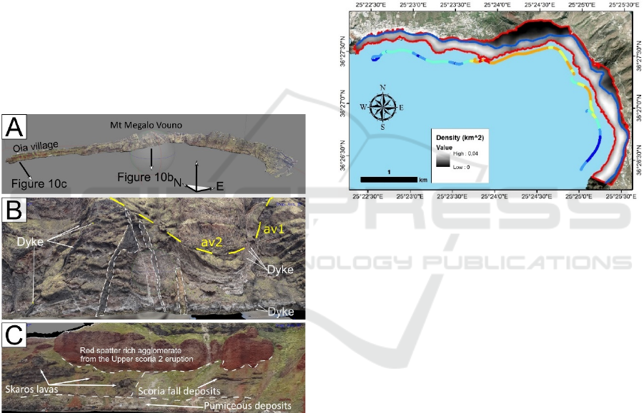
2 GEOLOGICAL BACKGROUND

The Santorini Volcanic Complex is located in the

Aegean Sea and represents the westernmost part of

the active Greek volcanic arc (Le Pichon and

Angelier, 1979). It is an active stratovolcano

composed of five islands (Fig. 1) that were initially

united, before multiple (at least four) caldera collapse

events formed the currently flooded caldera

morphology (Druitt, 2014) (e.g. Fig. 2a).

Figure 1: Satellite view of Santorini volcanic complex; the

major islands and volcanotectonic lineaments are shown

(CSK - Christiana-Santorini-Kolumbo).

Previous studies (Druitt et al., 1999; Rizzo et al.,

2015; Hooft et al., 2017) suggest the existence of

three volcanotectonic lineaments (Kameni line,

Kolumbo line and the Christiana-Santorini-Kolumbo

rift zone) which dissect the island and control magma

ascent in the shallow crust. Although volcanic

activity has been ceased since 1950, the 2011-2012

unrest episode showed magma accumulation beneath

the Nea Kameni island (Parks et al., 2012) while the

intense seismic activity along the Kameni V-T line

exhibited a possible resurgence which, however, did

not fed an eruption (Browning et al., 2015). The

stratigraphy of the northern part of the caldera wall

indicates a large sequence of effusive/explosive

subaerial volcanic activity with a variety of volcanic

products, and in particular lavas, scoria, tuffs and

hyaloclastites (Druitt et al., 1999) (Fig. 2b).

Figure 2: (A) View of the northern caldera wall; the Oia

village, as well as Mt Megalo and Kokkino Vouno, are

highlighted. (B) Dykes dissect the heterogeneous host rock.

Av1 unit: andesitic lavas, tuffs, breccia, and hyaloclastites.

Av3 unit: thinly bedded andesitic and basaltic lavas with

subordinate dacites, tuffs and scoria.

The basement lithologies belong to the Peristeria

stratovolcano (active 530-430 ka) and are capped by

the products of two later explosive cycles (360-3.6

ka). The Minoan Plinian eruption ignimbrite lies atop.

The dyke-fed eruptions are attested by a local radial

dyke swarm of ≥ 90 segments that are visible on the

caldera wall and reflect the magmatic and

volcanotectonic evolution of the volcano’s plumbing

system (Drymoni, 2020). The dykes follow variable

paths, and many cross-cutting relationships are

observed. Many arrested, deflected, and feeder-dykes

GISTAM 2021 - 7th International Conference on Geographical Information Systems Theory, Applications and Management

occur and dissect dissimilar mechanically layers

(Drymoni et al., 2020).

3 3D MODELLING

In this section, we describe the workflow through

which we applied the SfM techniques (e.g. Westoby

et al., 2012; Pepe and Prezioso, 2016; Bliakharskii

and Florinsky, 2018), which is subdivided into two

main steps: i) Boat survey and picture collection; and

ii) SfM photogrammetry processing. The final results

are provided in the form of VOs, DSMs, and an

Orthomosaic.

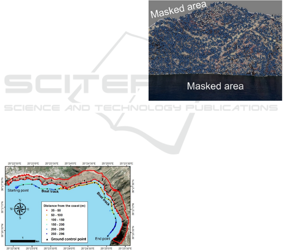
3.1 Boat Survey and Picture Collection

Instead of using a commercial UAV, we collected 887

pictures using a static camera, the Sony HX400V

bridge model, equipped with the Sensor CMOS

Exmor R® 1/2.3" (7.82 mm), 20.4 megapixel,

capable of providing GPS tagged photos (Geographic

coordinates/Datum WGS84), camera lens ZEISS

Vario-Sonnar® T* and φ55. The operator took the

pictures by keeping the camera parallel to the

“ground” and opposite to the caldera wall. Adjusted

camera settings were used, such as a Sport capture

mode and a constant focal length set to 4.34 mm. The

boat navigated along a 5.5 km track parallel to the

caldera wall from the W to the E-ESE, keeping a

constant speed of 4m/s (Fig. 3). The duration of the

boat survey was 25 mins, and the horizontal distance

range from the coastline was between 35.8 and 296.5

m (Fig. 3), with an average of 144.1 m (SD=70 m).

The Z value of each picture was corrected to a value

of 4.5 m a.s.l, resulting from GPS Real-time

kinematic (RTK) data recording.

Figure 3: Location of the collected pictures, with their

distance from the coast classified in 50m-length intervals.

The red curve highlights the area of interest, the boat track

is indicated by black arrows.

3.2 Photogrammetry Processing

The workflow continued with photogrammetry

processing. All pictures were managed through the

Agisoft Metashape (http://www.agisoft.com/)

photogrammetric software, which processes digital

images and generates 3D spatial data, providing a

high quality of point clouds (Burns et al., 2017). At a

general level, we followed the workflow used in

Bonali et al. (2020): i) picture alignment and sparse

cloud generation; ii) dense cloud building; iii) VO,

DSM and Orthomosaic generation. Firstly, the

pictures were uploaded and edited individually to

mask all the areas external to the caldera wall (sky

and sea) (Fig. 4), to achieve a better processing.

Figure 4: Masked picture; some commonly recognised

points by the software are also shown.

The next step consisted in getting an initial low-quality

photo alignment by considering only the measured

camera locations. Eventually, all the photos with

quality value ˂ 0.8 (or out of focus - visual revision)

were excluded from any further processing. To allow

for the co-registration of datasets and the calibration of

models resulting from SfM photogrammetry

processing, we added 50 Ground Control Points

(GCPs), (e.g. Westoby et al., 2012; James et al., 2017),

all provided with 1 m of accuracy. We considered the

latitude and longitude values from georeferenced aerial

photos and the elevation values from previous high-

resolution models designed by the National and

Kapodistrian University of Athens. After this step, we

re-processed the alignment to obtain better quality.

Regarding the alignment, we tested a total of 16

different approaches, considering the following

features: i) High and Medium accuracy; ii) Generic

and/or Reference preselection, as well as none of them;

iii) Key/Tie Point limit set to 40,000/4,000 and

100,000/10,000 respectively. For each, the dense cloud

Virtual Outcrops Building in Extreme Logistic Conditions for Data Collection, Geological Mapping, and Teaching: The Santorini’s Caldera

Case Study, Greece

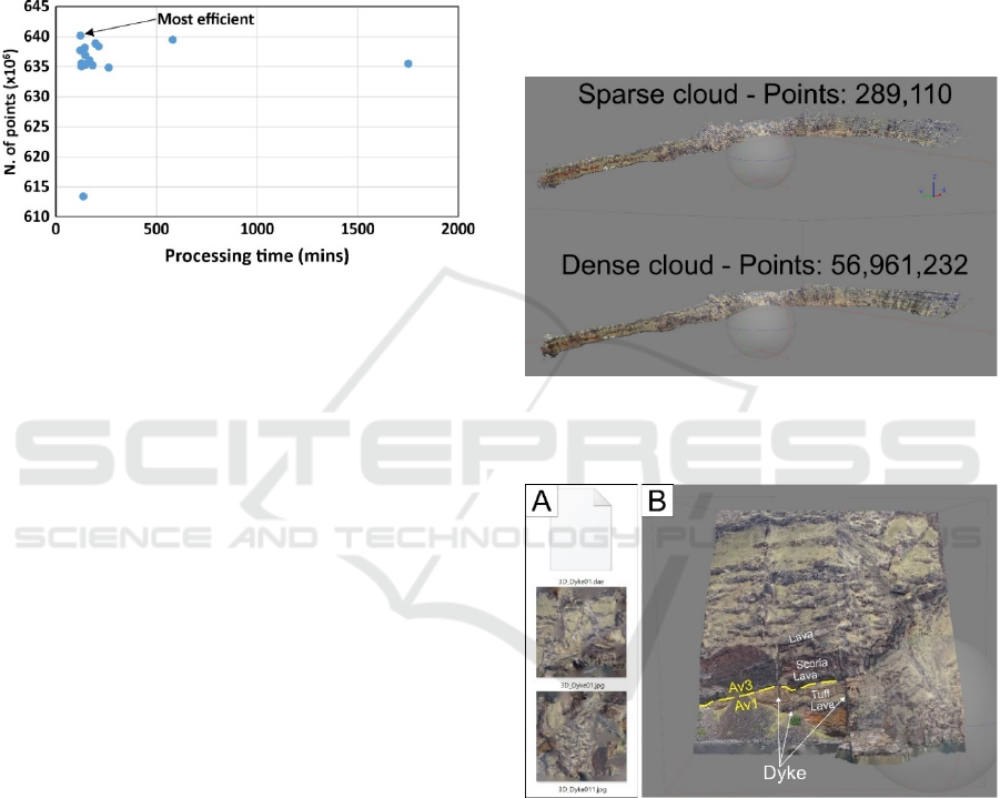
was generated with Medium accuracy and Mild depth

filtering. After these steps, we selected the most

efficient approach, considering the overall total length

of the processing time and the number of points of the

produced dense cloud. The most efficient approach to

generate the dense cloud was finally found to be the

Alignment with Medium accuracy and both Generic

and Reference selection activated (Fig. 5); the pictures

overlap ratio is always greater than 90%.

Figure 5: Graph showing the processing time vs the number

of dense cloud points, for the 16 different processing

approaches.

The duration of the aforementioned step was 121

mins, and the produced dense cloud had 63,770,936

points. Processing was performed using the Agisoft

Cloud beta service, from a virtual machine equipped

with the following features: a CPU-32 vCPU (2.7

GHz Intel Xeon E5 2686 v4), a GPU 2 × NVIDIA

Tesla M60, a RAM 240 GB. We also applied the

“Filter by Confidence” tool to remove noisy points

from the dense cloud. Primarily, we removed all the

points from the overall dense cloud in the range

between 0–1 and took out the ones which did not

relate to the final area and the model we wished to

obtain. On the resulting dense cloud, composed of

56,961,232 Points (Fig. 6), we first generated the

DSM model, where the Projection was set up to

WGS84 / UTM zone 35N, with interpolation both set

to disabled and enabled. Finally, we assigned the

Orthomosaic feature with the following “Average

setting” as Blending mode, and we kept the “Enable

hole filling” disabled, instead of the “Mosaic” as it is

usually done with UAV-captured pictures.

3.3 VOs Building

Regarding the VOs and the 3-D produced models, the

overall model was built as a tiled model with a Tile

size of 4096x4096 pixels and a medium face count.

This was suggested by Tibaldi et al. (2020), who

proposed to use the Tiled Model as a Virtual Reality

scenario. Some parts were also selected and shared

online for further dissemination activities. In detail, to

create VOs of adequate quality for online sharing, we

suggest the following steps. The first step is to build

the mesh from the dense cloud, with an Arbitrary 3D

surface type, and 2,100,000 number of faces.

Afterwards, it is necessary to create the texture, in two

separated files, with a tile size of 4096x4096 pixels;

then, the 3-D model can be exported in Collada file

format. The output is composed of three files, one for

the mesh (DAE file extension) and two for the texture

(jpg file extension) (Fig. 7a). The online shared model

is shown in Figure 7b.

Figure 6: Best sparse and dense cloud obtained with the

workflow mentioned above, including a “Filter by

confidence” tool.

Figure 7: (A) DAE file for the mesh and the two JPG files

of the texture feature needed for the 3D model (B). Av3 and

Av1 units as well as the dykes and the observed crustal

segment are explained in detail in the caption of Figure 2.

4 RESULTS

4.1 DSMs and Orthomosaic

We collected a total number of 877 pictures to be used

during the photogrammetry processing to build up the

DSM and the Orthomosaic. The size of the research

GISTAM 2021 - 7th International Conference on Geographical Information Systems Theory, Applications and Management

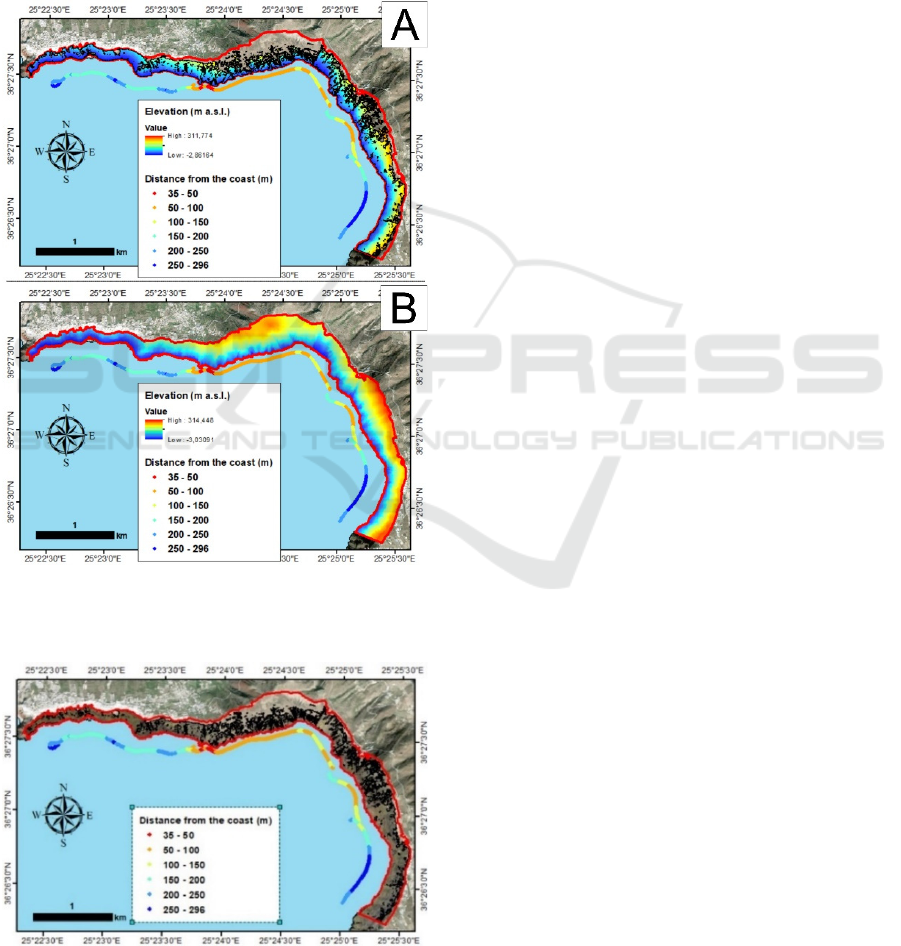
area was measured with the ArcGIS Pro tools and was

found to cover 1.84 km

(Fig. 3). The DSM,

processed without using interpolation settings,

covered an area of 1.25 km

, that is 30 % smaller than

the target area, resulting in a resolution of 22.3 cm/pix

and an elevation range from -2.68 to 311.77 m a.s.l.

(Fig. 8a). The DSM processed using interpolation

settings had the same pixel size, covered the entire

target area, and showed an elevation range from -3.0

to 314.5 m a.s.l. (Fig. 8b). The processing time of the

two DSMs was 3 mins and 22 mins, respectively.

Figure 8: DSMs derived by photogrammetry processing

limited to the target area (red area), built without (A) and

with interpolation settings selected (B).

Figure 9: Orthomosaic derived by photogrammetry

processing restricted to the target area (red area).

The 5-m-resolution DEM provided by the

National Cadastre & Mapping Agency S.A. is in the

range of 2.20 - 329.23 m a.s.l.. Regarding the

Orthomosaic, it has the same areal coverage as the

first DSM, no interpolation settings were selected,

and has a resolution of 5.8 cm/pix (Fig. 9). Its

processing time was 493 mins. To define the research

area, we first calculated a ridgeline. We used the 5-m-

resolution digital elevation model (DEM) derived

from the area's orthophoto map (2012) of the National

Cadastre & Mapping Agency S.A. in ArcGIS Pro, to

create the flow direction initially and then the flow

accumulation raster files by applying the DINF

method, that uses the steepest slope of a triangular

facet. Then, we reclassified the flow accumulation

file into two classes separating the zero value areas

from the rest, isolating the ridgeline area. We then

converted the reclassified raster file to a vector one,

creating the required ridgeline. Finally, using the

orthophoto map of the area, we modified the ridgeline

as well as the coastline excluding the residential

areas.

4.2 3-D Tiled Model and VOs

We produced the overall 3D Tiled model in 270 mins,

and the texture resolution was similar to the

Orthomosaic value, i.e. 5.8 cm/pix (Fig. 10a).

Similarly to the DSMs and the Orthomosaic, in terms

of planar areal extent, the covered area is the same.

However, differently from the Orthomosaic and the

DSMs, in the 3D Tiled Model all the vertical parts of

the caldera, which could be mapped on 2D models,

are very well represented, as shown in detail in Figs.

10b-c and from the VO displayed in Figure 7b.

4.3 Relationship between Camera

Location and the Derived Models

Even though this is a first approach, our models

generally showed a positive correlation between the

operator-coast distance and the most representative

elevation values in the derived DSM (no interpolation

- Fig. 8a). However, in the western and southeastern

part of the caldera, the images were collected from a

longer distance, so the elevation values were

portrayed in a better way (both in terms of their areal

coverage and maximum elevation) in the produced

DSM and complied with specific conditions. These

conditions allowed us to estimate the most

representative operator-coast distance vs best-

performed elevation above sea level solutions which

were: i) for ≤100m operator-coast distance, elevation

values were between 0-60m, ii) for 100-200m

Virtual Outcrops Building in Extreme Logistic Conditions for Data Collection, Geological Mapping, and Teaching: The Santorini’s Caldera

Case Study, Greece

operator-coast distance, a maximum elevation of 150-

200m could be reached, iii) for >200m operator-coast

distance the elevation values could be suitable for the

whole model (313m maximum vertical altitude). The

above specifications are crucial to plan further similar

field campaigns in such extreme conditions.

Therefore, we designed a protocol to preliminarily

describe the relationship between these realistic field

parameters (operator-caldera distance and elevation),

which can still be improved. First, we calculated the

point density of the DSM data. Then, we selected an

upper elevation limit value wherever the derived

density was high (0.02 km

;

Fig. 11). This allowed the

model to trace the most representative solutions. We

used such limit as a parameter towards the minimum

net (3D) distance calculation between this upper limit

and the camera, with information sampling each 1 m

along the line (Fig. 11). We show this relationship in

Figure 12, where the Maximum Elevation reachable

(y-axes) is a function of the 3D distance multiplied by

0.4393 minus 1.7881.

Figure 10: (A) The resulting 3D Tiled Model. (B) 3D model

view of the area below Mt Megalo Vouno. The dykes were

emplaced into a heterogeneous and anisotropic host rock,

which belongs to the oldest local volcanic activity

(Peristeria stratovolcano, 530-430 ka), and dissected the

bottom units: i) av1 - a mixture of andesitic lavas, tuffs,

breccias, and hyaloclastites; ii) av2 - silicic andesitic lavas.

5 DISCUSSION

Here, we critically discuss the application of our

proposed methodological approach to the VOs,

DSMs and Orthomosaic design in extreme conditions

where the use of UAVs is difficult for image

collection. We have designed a safe, user-friendly,

economic and well-developed approach to build up

3D models aimed at overcoming field-related

challenges but, most importantly, tackling the

technical limitations and methodological impact on

the interpretation of the findings, which could not be

addressed by other techniques. Our well-tested

methodology proposes that the resolution produced

by the SfM-derived DSMs and Orthomosaic is well

portrayed and successfully serves the scopes of

geological interpretation and quantitative and

qualitative data collection for geoscientists.

Figure 11: Map showing the point density values calculated

by the DSM, with no interpolation settings. The blue line

represents the upper elevation selected limit.

We also critically consider that the difference

between the 5-m DSM and the SfM derived model

(interpolation settings were inactive) can produce

good correlations for the used scale (km range) of our

study. Our results show a major difference between

the elevation values produced by the two models (Fig.

13), ranging from -63.19 to 52.32 m, mean value =

-0.09. However, their statistical analysis implies a

much lower standard deviation (SD) value than its

broad range, suggesting instead that the majority of

data are within an SD of 9.95. To obtain results with

a better statistical performance, we propose an

updated scenario which offers: 1) high precision

GCPs, 2) a UAV-based mission in conjunction with

this methodology to complement the collected picture

set considering different cliff and elevation angles.

This can increase the quality of the produced DSM

and provide more accurate structural data. We have

also tested an identical scenario and have designed a

DSM by activating the interpolation settings. The

statistical analysis shows a broader range of values as

well as a greater standard deviation (SD) than in the

previous case; the range is between -62.44 and 98.56,

GISTAM 2021 - 7th International Conference on Geographical Information Systems Theory, Applications and Management

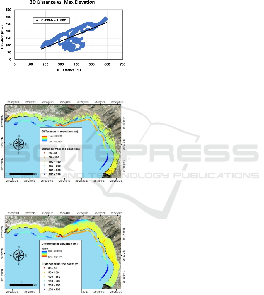
the mean is 3.02 and the SD = 13.24 (Fig. 14).

Furthermore, we noticed that both the over and

underestimated elevation values belonged to pictures

collected very close to the coast.

Figure 12: Graph showing the relation between the 3D

distance from the camera and the maximum reachable and

reliable elevation in the DSM.

Figure 13: Raster showing the difference in elevation

between the 5-m DSM and the SfM-derived DSM obtained

with no interpolation settings.

Figure 14: Raster showing the elevation difference between

the 5-m DSM and the SfM-derived DSM obtained with

active interpolation setting.

Finally, although the Orthomosaic suffered from

significant distortion effects due to the high slope

morphology of the target area, the 3D Tiled model, as

well as the selected VOs, show some excellent

vertical outcrops. The above considerations prove

that the proposed technique can be used for research

surveys and data collection protocols; such activities

were once instead impossible to carry out with

sufficient precision, owing to accessibility limitations

(e.g. Fig. 7). For example, our methodology gave

satisfying results in relation to the quantitative

measurements of dyke thickness, as shown in Figs. 2b

and 7. The data of this campaign and especially the

ones related to dyke thickness measured by Drymoni

et al. (2020) in Figs 2b and 7 have been compared

with our derived 3D model, showing excellent

overlap. Similarly, we refer to the comparisons

between another dyke studied by Tibaldi et al. (2020)

and our 3D model. The results show, once again, a

centimetric difference between the two thickness

measurements. Such observations suggest the

practicality, but most importantly the level of

confidence of the SfM-derived 3D models proposed

here, for data collection and 3D geological

reconstructions. Finally, the overall 3D models, as

well as their selected parts, can be excellent teaching

resources and could serve significantly as part of

interactive outreach activities. In this regard, we aim

to enhance the accessibility of the northern caldera

wall, publishing three sites as “Virtual Outcrops”

(e.g. Pasquaré Mariotto et al., 2020) available on the

webpages: https://geovires.unimib.it/geovolc/ and

https://geovires.unimib.it/shallow-magma-bodies/,

where a scientific description is also provided for

each model. Finally, as suggested by Tibaldi et al.

(2020), the SfM-derived 3D Tiled model can be

imported in a game engine, building fully navigable

immersive VR systems (https://www.geavr.eu/).

6 CONCLUSIONS

In the present work, we achieved the following

outcomes: i) a major, high-resolution 3D tiled model

with a texture resolution of 5.8 cm/pix, ii) two DSMs

and an Orthomosaic with a pixel resolution of 22.3

and 5.8 cm/pix respectively, iii) a series of VOs for

dissemination activities. More importantly, we

applied the aforementioned SfM photogrammetry

approach in extreme conditions, providing a

preliminary equation that can be used to plan further

surveys along the almost vertical and inaccessible

cliff, using a static camera to run the pictures

collection task.

Virtual Outcrops Building in Extreme Logistic Conditions for Data Collection, Geological Mapping, and Teaching: The Santorini’s Caldera

Case Study, Greece

ACKNOWLEDGEMENTS

Funding is from : i) the ILP-Task Force II (Leader A.

Tibaldi); ii) the MIUR project ACPR15T4_00098–

Argo3D (http://argo3d.unimib.it/); iii) the Virtual

Diver project (https://www.virtualdiver.gr/); iv)

NEANIAS project (https://www.neanias.eu/). Special

thanks to Captain Giorgos Renieris of the Santorini

Boatmen Union. Agisoft Metashape is acknowledged

for photogrammetric data processing. Finally, this

paper is an outcome of GeoVires lab

(https://geovires.unimib.it).

REFERENCES

Bliakharskii, D. P., & Florinsky, I. V. (2018, March).

Unmanned aerial survey for modelling glacier

topography in Antarctica: first results. In GISTAM (pp.

319-326).

Bonali, F. L., Tibaldi, A., Corti, N., Fallati, L., & Russo, E.

(2020). Reconstruction of Late Pleistocene-Holocene

Deformation through Massive Data Collection at Krafla

Rift (NE Iceland) Owing to Drone-Based Structure-

from-Motion Photogrammetry. Applied Sciences,

10(19), 6759.

Browning, J., Drymoni, K., Gudmundsson, A., (2015).

Forecasting magma-chamber rupture at Santorini

volcano, Greece. Scientific reports, 5, 15785.

Burns, J. H. R., & Delparte, D. (2017). Comparison of

commercial structure-from-motion photogrammety

software used for underwater three-dimensional

modeling of coral reef environments. The International

Archives of Photogrammetry, Remote Sensing and

Spatial Information Sciences, 42, 127.

Druitt, T.H., Edwards, L., Mellors, R.M., Pyle, D.M.,

Sparks, R.S.J., Lanphere, M., Davis, M., Barriero, B.,

(1999). Santorini Volcano. Geological Society Memoir

No. 19, 165.

Druitt, T. H., (2014). New insights into the initiation and

venting of the Bronze-Age eruption of Santorini

(Greece), from component analysis, Bull. Volcanol.,

76, 794

Drymoni, K., Browning, J., Gudmundsson, A., (2020).

Dyke-arrest scenarios in extensional regimes: Insights

from field observations and numerical models,

Santorini, Greece, Journal of Volcanology and

Geothermal Research, 396, 106854

Drymoni, K., (2020). Dyke propagation paths: The

movement of magma from the source to the surface,

PhD thesis, Royal Holloway University of London, UK

Fallati, L., Saponari, L., Savini, A., Marchese, F., Corselli,

C., & Galli, P. (2020). Multi-Temporal UAV Data and

object-based image analysis (OBIA) for estimation of

substrate changes in a post-bleaching scenario on a

maldivian reef. Remote Sensing, 12(13), 2093.

Friedrich, W., Kromer, B., Friedrich, M., Heinemeier, J.,

Pfeiffer, T., Talamo, S., (2006). Santorini eruption

radiocarbon dated to 1627–1600 Bc., Science, 312, 548

Gudmundsson, A., 2020. Volcanotectonics. Cambridge

University Press, Cambridge.

Hooft, E.E.E., P. Nomikou, D.R. Toomey, D. Lampridou,

C. Getz, M. Christopoulou, D. O’Hara, G.M. Arnoux,

M. Bodmer, M. Gray, B.A. Heath, and B.P. Vander

Beek, (2017). Backarc tectonism, volcanism, and mass

wasting shape seafloor morphology in the Santorini-

Christiana-Amorgos region of the Hellenic Volcanic

Arc, Tectonophysics, 712-713, 396-414.

James, M. R., Robson, S., & Smith, M. W. (2017). 3‐D

uncertainty‐based topographic change detection with

structure‐ from‐motion photogrammetry: precision

maps for ground control and directly georeferenced

surveys. Earth Surface Processes and Landforms,

42(12), 1769-1788.

Le Pichon, X., Angelier, J., (1979). The Hellenic arc and

trench system: A key to the neotectonic evolution of the

eastern Mediterranean area. Tectonophysics, 60, 1-42.

Pasquaré Mariotto, F., Bonali, F. L., & Venturini, C.

(2020). Iceland, an open-air museum for geoheritage

and Earth science communication purposes. Resources,

9(2), 14.

Parks, M.M., Biggs, J., England, P., Mather, T.A.,

Nomikou, P., Palamartchouk, K., Papanikolaou, X.,

Paradissis, D., Parsons, B., Pyle D.M., (2012).

Evolution of Santorini Volcano dominated by episodic

and rapid fluxes of melt from depth, Nat. Geosci., 5,

749-754.

Pepe, M., & Prezioso, G. (2016, April). Two Approaches

for Dense DSM Generation from Aerial Digital Oblique

Camera System. In GISTAM (pp. 63-70).

Rizzo, A.L., Barberi, F., Carapezza, M.L., Di Piazza, A.,

Francalanci, L., Sortino, F., D’Alessandro, W., (2015).

New mafic magma refilling a quiescent volcano:

Evidence from He–Ne–Ar isotopes during the 2011–

2012 unrest at Santorini, Greece. Geochemistry,

Geophysics, Geosystems, 16, 798- 814.

Scott, C., Bunds, M., Shirzaei, M., & Toke, N. (2020).

Creep along the Central San Andreas Fault from

Surface Fractures, Topographic Differencing, and

InSAR. Journal of Geophysical Research: Solid Earth,

125(10), e2020JB019762.

Tibaldi, A., & Bonali, F. L. (2017). Intra-arc and back-arc

volcano-tectonics: Magma pathways at Holocene

Alaska-Aleutian volcanoes. Earth-Science Reviews,

167, 1-26.

Tibaldi, A., Bonali, F. L., Vitello, F., Delage, E., Nomikou,

P., Antoniou, V., & Whitworth, M. (2020). Real world–

based immersive Virtual Reality for research, teaching

and communication in volcanology. Bulletin of

Volcanology, 82(5), 1-12.

Xu, X., Aiken, C.L., Nielsen, K.C., (1999). Real time and

the virtual outcrop improve geological field mapping.

Eos, Transactions American Geophysical Union,

80(29), 317-324.

Westoby, M. J., Brasington, J., Glasser, N. F., Hambrey, M.

J., & Reynolds, J. M. (2012). ‘Structure-from-

Motion’photogrammetry: A low-cost, effective tool for

geoscience applications. Geomorphology, 179, 300-314.

GISTAM 2021 - 7th International Conference on Geographical Information Systems Theory, Applications and Management