
Deep Learning Application for
Urban Change Detection from Aerial Images
Tautvydas Fyleris
1
, Andrius Kriščiūnas
2
, Valentas Gružauskas
3
and Dalia Čalnerytė
2
1
Kaunas University of Technology, Faculty of Informatics, Department of Software Engineering, Lithuania
2
Kaunas University of Technology, Faculty of Informatics, Department of Applied Informatics, Lithuania
3
Kaunas University of Technology, School of Economics and Business, Sustainable Management Research Group, Lithuania
Keywords: Urban Change, Aerial Images, Deep Learning, JEL: O18, C45, C55.
Abstract: Urban growth estimation is an essential part of urban planning in order to ensure sustainable regional
development. For such purpose, analysis of remote sensing data can be used. The difficulty in analysing a
time series of remote sensing data lies in ensuring that the accuracy stays stable in different periods. In this
publication, aerial images were analysed for three periods, which lasted for 9 years. The main issues arose
due to the different quality of images, which lead to bias between periods. Consequently, this results in
difficulties in interpreting whether the urban growth actually happened, or it was identified due to the incorrect
segmentation of images. To overcome this issue, datasets were generated to train the convolutional neural
network (CNN) and transfer learning technique has been applied. Finally, the results obtained with the created
CNN of different periods enable to implement different approaches to detect, analyse and interpret urban
changes for the policymakers and investors on different levels as a map, grid, or contour map.
1 INTRODUCTION
Urban planning is an essential economic activity for
regions seeking to maintain prosperity. It is essential
to identify urban growth patterns to be able to provide
recommendations for infrastructure planning. One
approach might be waiting for an area to expand and
plan the infrastructure later; however, in this case, the
cost of the projects might increase. An alternative
approach could be estimating future urban growth
patterns and planning infrastructure projects in
advance. Proper preparation for such projects could
increase the sustainability of the region in terms of
social benefit and economic growth potential. In
addition, the identified urban growth patterns can also
be used by private companies to plan investment
strategies, not limiting to government institutions.
Urban growth analysis can be conducted using
different data sources and methodologies. For
instance, social-economic indicators of the region
could be analysed to estimate the demographic
change. However, this kind of data mainly focuses on
the temporal aspects, with a limited focus on spatial
ones. Thus, for urban growth analysis, remote sensing
data can be used more effectively. Remote sensing
data consists of satellite images, radar images, aerial
images, etc. A comprehensive overview of remote
sensing data for economics has been provided by
(Donaldson & Storeygard, 2016). To detect change in
remote sensing data, mainly two approaches are used.
One approach is unsupervised learning, which
focuses on change detection of pixels without clearly
identifying the types of detected objects. Similar
applications have been conducted in video analysis,
which focuses on unsupervised learning, i.e. change
of individual pixels, rather than recognition of the
specific object. Goyette et al. (2012) created a dataset
for testing change algorithms in videos. This dataset
has been widely used to develop algorithms (Goyette
et al., 2012). Kanagamalliga and Vasuki (2018)
proposed a video flow analysis approach, in which
firstly the background is extracted and later the
contour of the movable object is determined
(Kanagamalliga & Vasuki, 2018). Wang et al. (2019)
developed a motion tracking algorithm based on
tubelet generation, which compares the change in
frames to improve the video object detection (B.
Wang et al., 2019). Similar approaches have been
previously developed to evaluate change and monitor
the disturbances in satellite images based on
vegetation index, which is suitable for disaster
monitoring (Verbesselt et al., 2010; Verbesselt et al.,
2012). Similar change detection methods have also
Fyleris, T., Kriš
ˇ
ci
¯
unas, A., Gružauskas, V. and
ˇ
Calneryt
˙
e, D.
Deep Learning Application for Urban Change Detection from Aerial Images.
DOI: 10.5220/0010415700150024
In Proceedings of the 7th International Conference on Geographical Information Systems Theory, Applications and Management (GISTAM 2021), pages 15-24
ISBN: 978-989-758-503-6
Copyright
c
2021 by SCITEPRESS – Science and Technology Publications, Lda. All rights reserved
15

been tested with satellite images. For example, Celik
(2009) proposed principal component analysis and k-
mean clustering to develop an unsupervised change
detection algorithm (Celik, 2009). Jong and Bosman
(2019) developed an unsupervised change detection
algorithm by using convolutional neural networks (de
Jong & Sergeevna Bosman, 2019).
Another approach is to use supervised learning
and detect precise objects from remote sensing data,
such as roads, buildings, forests, etc. For example,
Wang et al. (2015) proposed a deep learning approach
to extract road networks from satellite images (J.
Wang et al., 2015). Nahhas et al. (2018) developed a
deep learning approach for building detection in
orthophotos (Nahhas et al., 2018). Langkvist et al.
(2016) integrated satellite images with digital surface
models to improve per-pixel classification of
vegetation, ground, roads, buildings, and water
(Längkvist et al., 2016). Marmanis et al. (2016)
developed a deep learning algorithm for aerial image
classification with a 88.5% accuracy (Marmanis et
al., 2016). Transfer learning is also widely applicable
in remote sensing area. Xie et al. (2016) extracted
light intensity of satellite images, validated the
approach with respect to the survey data, used transfer
learning to train the model on known data and applied
it to estimate poverty levels in Uganda (Xie et al.,
2016). Wurm et al. (2019) used a similar approach of
transfer learning to estimate slums. The initial model
was trained on high quality satellite images of
QuickBird and transferred to Sentinel-2 images,
which allowed for gaining higher accuracy in
estimating slums (Wurm et al., 2019). After
identifying the objects in remote sensing data, they
can be combined with various social-economic
indicators, thus reducing the costs of surveys. Jean et
al. (2016) developed a machine learning approach to
predict poverty from satellite images. The approach
integrated the deep learning model with survey data,
which helped reduce the costs and increase the
accuracy of social demographic indicators (Jean et al.,
2016). Suraj et al. (2018) developed a machine
learning algorithm to monitor the development
indicators from satellite images (Suraj et al., 2018).
In summary, it can be stated that most of the
publications focus on detection of specific object at a
micro level in high resolution images. For the lower
resolution images (e.g. Copernicus), research is
mainly conducted on recognition of the type of land
use (e.g. agriculture land). Usually these images are
integrated with radar images and focus on reflection
analysis. Only a limited number of studies been
identified, in which analysis for a time-series of
images at a country level is performed. In most of
them, limited information on the methodological
approach and possible issues is provided. Thus, our
publication focuses on filling this gap.
In this publication, we focus on extraction of
indicators from a time series of visual information in
relation to geospatial data. The difficulty in analysing
a time series of remote sensing data lies in ensuring
that the accuracy stays stable in different periods. For
instance, if one period of aerial images has an
accuracy of 90%, and another of 86%, it would be
unclear whether the urban change actually happened,
or it was calculated due to the error of the machine
learning (ML) model. Thus, it is important to ensure
consistent accuracy of object detection between
different periods. In this paper, the available dataset
of the same geographical region in different time
periods was of different quality due to the image
spectrum and resolution. This was caused by the fact
that with time, technical capabilities enabled attaining
better quality (i.e. before 2000, visual data for the
same region was available only in grey scale
compared to the current RBG of 16 bit depth).
Moreover, the ground truth data may vary due to the
time delay between the real actions, which are visible
in real time and data input to registers or external
databases. To overcome these limitations, transfer
learning technique has been applied. The initially pre-
trained DeepLabv3 model with a ResNet50 backbone
trained on the ImageNet data has been selected. Next,
model adjustment has been carried out in two steps,
with coarse and fine-tuning datasets. The coarse
dataset was created automatically by randomly
selecting different locations and merging it with the
labels of Open Street Map. The fine-tuning dataset
was created according to the same principles;
however, the images were manually reviewed by
removing those, for which the labelled data did not
meet the actual visible data. Finally, to ensure that the
model of different periods provides similar accuracy,
we normalised all datasets according to the one of the
worst quality (oldest in time) and the fine-tuning
operation for different time periods was performed
for separate models, where loss behaviour was
tracked for the sub-model of each period.
Incidentally, such strategy allows to better adapt each
sub-model for the variances of photo in different
periods, i.e. seasons, times of the day, etc.
Afterwards, results obtained with the created ML
model of different periods will enable to implement
different approaches to detect, analyse and interpret
urban changes for policy makers and investors. This
means that the approaches used to analyse the parsed
data may be applied on different levels, i.e. on the
finest level, the processed data can be seen as a map.
GISTAM 2021 - 7th International Conference on Geographical Information Systems Theory, Applications and Management
16
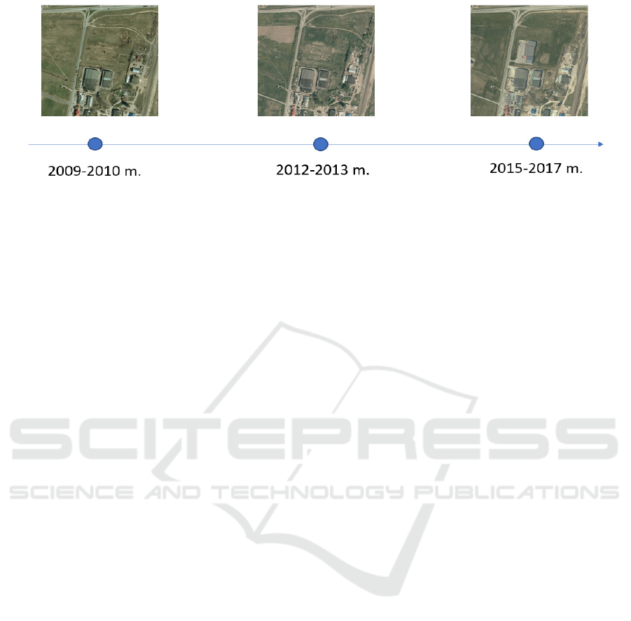
Figure 1: Example of view difference at the same place in different periods.
On the middle level, the difference of the indicator
can be analysed to easily detect the change of the
selected indicator in grid cells and their clusters. On
the highest level, the change of the indicator can be
presented as a contour map.
2 METHODOLOGY AND DATA
ANALYSIS
2.1 Methodology Overview and
Selection of Dataset
The idea that urban changes in time can be
determined by the view visible in aerial photos is
demonstrated by the example, where the number of
buildings at same place differs (see Fig 1).
A different speed of changes of buildings, forests,
land use, etc. in the regions may result in different
development speed of the region. Visual data of
Lithuania has been selected for the analysis of the
relationship between the information obtained using
computer vision to track and interpret the visual
information (raster graphics). The research focuses on
two main objectives:
a) to create a machine learning (ML) model,
which enables to obtain interpretable values
on the country level in different time periods
and to analyse them on a granular level;
b) to perform an analysis of the ML model results
according to its suitability for the
identification of different urban growth
patterns.
Different data sources for analysis have been
investigated. Firstly, Copernicus Sentinel Missions
was considered as a data source. However, after
serious consideration it yielded the following
problems:
low resolution for building segmentation
and initial tests demonstrated bad results;
only recent data is stored, and historical
data is not available.
Admittedly, there are several methods to improve
the model accuracy, e. g. Shermeyer and Etten (2019)
applied super-resolution to satellite images and
concluded that super-resolving native 30 cm imagery
to 15 cm yielded the best results of 13 – 36%
improvement when detecting objects (Shermeyer &
Van Etten, 2019). The image can be also enhanced
using a discrete wavelet transform as was done in the
study of Witwit et al. (2017) (Witwit et al., 2017).
Furthermore, studies have been conducted where
Sentinel 2 data was used to classify the building areas
of the ground
(Krupinski et al., 2019), (Corbane et al.,
2020); however, due to a wider period of data and
better quality, ORT10K was chosen as an alternative
source for this study. The first period data resolution
of ORT10K was 0.5 m x 0.5 m and 8 bit RGB depth
(7 bit effective), for the second and third periods,
image resolution increased to 0.25 m x 0.25 m per
pixel, while the colour depth for the second period
was 8 bit RGB and 16 bit for the third. The principal
scheme of the research is shown in Fig. 2. The
detailed steps of analysis are described in the
following chapters.
2.2 Computer Vision Model
Dataset Preparation and Normalisation. The
ORT10LT contains 3 periods of country-specific
visual information. For labelling (indicators), the
Open Street Map (OSM) data source was chosen as
ground truth. Automatic query OSM database was
used for labelling. Technically, the process can be
described as follows: the ORT10LT segments were
cut by the chosen geographic points in the country
and then labelled directly from the OSM database
(Fig. 3).
Deep Learning Application for Urban Change Detection from Aerial Images
17
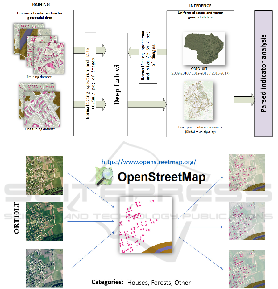
Figure 2: Principal scheme of the ML model construction and extraction of interpretable indicators.
Figure 3: Dataset preparation.
The OSM data has a lot of categories; however, in
this research, only 3 categories have been selected:
houses, forests and other. Water and road categories
have also been considered for inclusion into the
model, but due to the fact that the photos were taken
in different seasons (spring/summer), it was
concluded that the river flood might affect the water
area significantly. Moreover, while using RGB only,
water in some regions can be hard to distinguish from
vegetation (green water). The road category was left
out due to the fact that OSM mapping data defines
roads only as lines (not polygon): although the width
of the road can be technically guessed from the data,
it is not always correct. Finally, following the dataset
analysis, two types of problems were identified in the
selected dataset:
logical – the OSM data does not always
match the photos due to mistakes in
mapping or changes in the environment;
quality – the results for photos taken in
different periods or locations may vary due
to their quality:
GISTAM 2021 - 7th International Conference on Geographical Information Systems Theory, Applications and Management
18
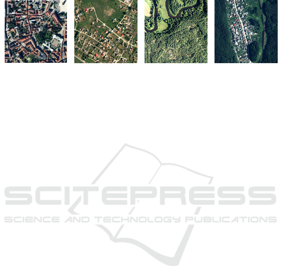
a
b
c
d
Figure 4: a, b) image selected with a house centred; c, d) image selected randomly.
(a) images were taken at a different time of the
day, which results in varying lighting (early
morning vs noon);
(b) subtle angle differences between photos;
(c) the equipment used to capture the images in
different location differs (different colour
response and dynamic range; the captured
images are blurry due to the fact that the
photos were taken early in the morning or at
night).
The logical problem has been solved in the dataset
preparation stage. The training dataset image size
chosen was 1024x1024 pixels (the main constraint
being the GPU memory limit). To avoid the initial
bias in the dataset distribution, when e.g. only rural
areas are selected for the initial training dataset, the
dataset was prepared according to the indicators
(houses, vegetation), which would be analysed in the
next stage. The first part of the dataset was created by
picking a random building from the OSM database
and focusing it in the middle of the input image. The
second part was constructed by applying the same
technique where random points for the whole country
have been selected. Finally, for the coarse dataset,
5,000 images have been selected (4,000 with
buildings and 1,000 with vegetation, covering a total
area of 1,250 km
2
). Different techniques of initial
image selection and a relatively large number of
images allow for ensuring that different cases are
covered for the whole country dataset. Examples of
different parts are provided in Fig. 4.
The fine-tuning dataset was created according to
the same principles; however, the images were
manually reviewed by removing the ones, for which
the labelled data did not meet the actual visible data.
Ultimately, 320 images (210 with buildings and 110
with vegetation, covering a total area of 80 km
2
) were
selected.
To solve the problems related to the different
quality of images, normalisation procedure was used
as follows:
a) resolution was normalised to 0.5 m/pixel;
b) contrast was normalised using a 2%–98%
percentile interval; all pixels over and under
the interval were clipped to minimum or
maximum values;
c) standard computer vision normalisation
procedure was applied (mean=[0.485, 0.456,
0.406], std=[0.229, 0.224, 0.225]).
Model Training and Result Analysis on the Finest
Level. Various models and visual analysis methods
can be used for object detection, segmentation, or
instance segmentation (Längkvist et al., 2016; Liu et
al., 2020; Marmanis et al., 2016; Wurm et al., 2019).
The argumentation for selecting the model deals with
the computational restriction to be able to analyse the
whole country in different periods. For this reason,
DeepLab3 with a ResNet50 backbone was chosen
(the main prerequisite being to be able run on limited
VRAM devices: NVIDIA RTX 2080ti with 11GB
RAM). The loss function was changed from Softmax
entropy loss to focal loss (Corbane et al., 2020) due
to the nature of data, absence of labels and
mislabelled areas (for example, areas without
buildings, or just background). Focal loss is an
alternative approach to loss function, which focuses
on misclassified examples and imbalanced data (such
as representing a single class in the entire detection
region, for example, forest only) and yields good
practical results. Formally, focus loss 𝐹𝐿
𝑝
can be
defined by the following equation:
𝐹𝐿
𝑝
𝛼
1𝑝
𝑙𝑜𝑔
𝑝
(1)
where 𝛼 is for 𝛼 - balanced form to reduce impact
for detection outliners; 𝛾 – is the focal factor. When
𝛾 = 0, focal loss is the same as cross-entropy loss;
however, with higher 𝛾 values, the loss reduces the
impact of easy examples and scales down the total
Deep Learning Application for Urban Change Detection from Aerial Images
19
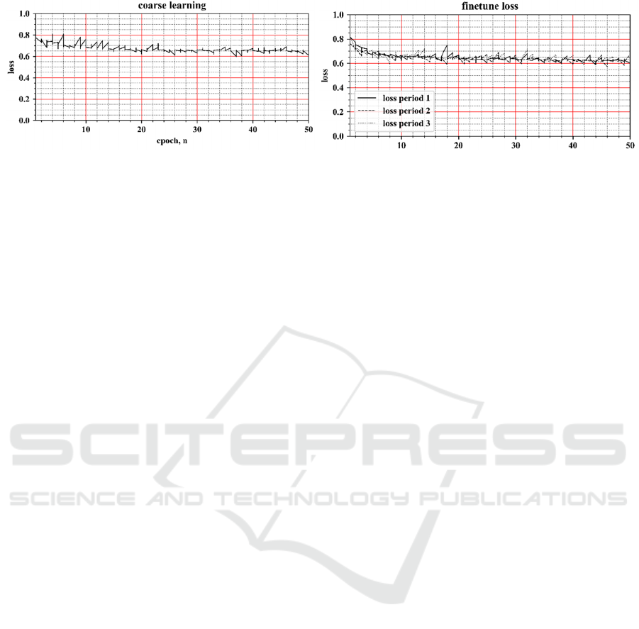
a
b
Figure 5: a) coarse learning loss; b) fine-tuning losses for 3 periods using fine-tuning.
loss value, which in turn increases the probability of
correcting misclassified examples. The class
classification function 𝑝
has the following definition:
𝑝
𝑝𝑖𝑓𝑦1
1𝑝 𝑜𝑡ℎ𝑒𝑟𝑤𝑖𝑠𝑒
(2)
where 𝑦 specifies the ground truth class 𝑦 ∈ {±1}
and 𝑝 ∈[0,1] is the model probability for the class. For
this experiment, 𝛼 =0.25 and 𝛾=2.
The technical specifications of the selected model
are as follows:
input layer: 1024 x 1024 pixels (result
taken from 896 x 896 pixels) ~ 448 m x
448 m (or ~0.2 km
2
) area;
coarse learning: learning rate 0.5e-3;
momentum 0.5; 5,000 samples per epoch;
fine-tune: learning rate 5e-05; momentum
0.1; 100 samples per epoch.
The mean value of focal loss (1) during the
training process of the model is provided in Fig 5
From the training process (see Fig. 5.) it can be
seen that the initial model with the coarse dataset
converges slower compared to models with the fine-
tuning dataset. Furthermore, all models for the fine-
tuning operations start from a similar loss function
value and correspond to the initial one of the coarse
dataset. It could be explained by the fact that errors in
the test vector of the coarse dataset compared to the
correctly labelled parts do not outweigh the errors in
different periods. In addition, it can be clearly seen
that the single model for each time period works
better with the fine-tuning dataset, for which the
incorrectly labelled data has been removed. Such
model separation strategy for each period provides
two valuable properties. On the one hand, if, in the
model training process, the image quality
normalisation process between periods leaves some
shortcomings and the image still has differences due
to its technical quality or seasonality between the
periods, then the model adapts easier to the photo
specifics, the dataset necessitating revision for the
model training is smaller, and better final results can
be obtained. On the other hand, the model training
results can be compared between different periods to
validate that models work well for different periods
and provide similar results, which allow for
comparison of results of different time periods. In
case of a bias of building detection between periods,
the quality of normalisation should be taken into
account, or correction coefficients could be applied to
minimise the bias.
3 ANALYSIS OF RESULTS
Finally, the model has been developed using 3 main
indicators. The direct results obtained with the
developed model of different periods enabled to
analyse and interpret the results on different levels.
Firstly, the analysis of urban change could be
conducted on the country level.
The buildings detected in the aerial images can be
depicted as polygons scattered through the region.
From this information, it is possible to create a plot
for spatial distribution by using kernel density. Fig. 6.
shows the kernel distribution of buildings identified
in the last period of images (year 2015 – 2017). The
figure represents the whole Lithuania, which area is
65,300 km². The distribution clearly identified the
major cities of Lithuania, i.e. Vilnius, Kaunas,
Klaipėda, Panevėžys, and Šiauliai.
On the middle level, it is possible to identify more
clearly the change of the region by creating a heat
map. For the creation of the heat map, the country was
divided into a grid, with the identification of the total
number of buildings detected per grid. Then, the
difference between the periods and grids was
obtained.
GISTAM 2021 - 7th International Conference on Geographical Information Systems Theory, Applications and Management
20
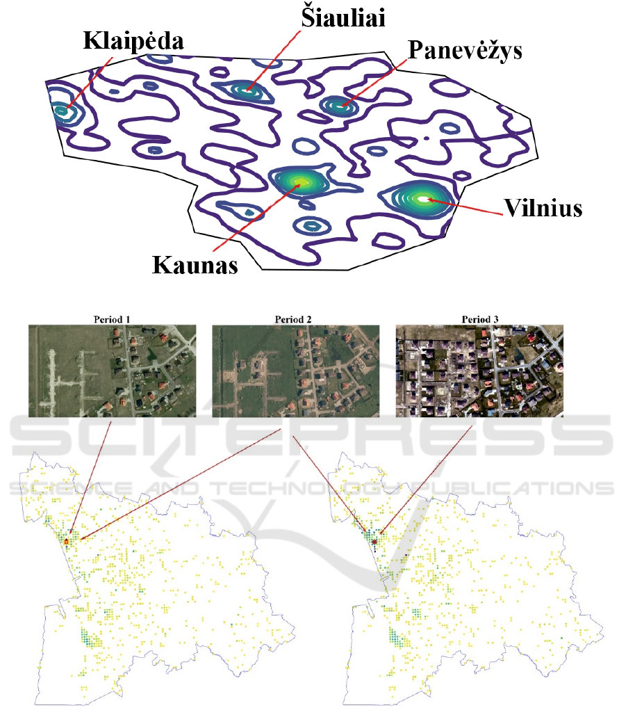
Figure 6: Kernel density plot of the detected buildings.
a
b
Figure 7: Heat map of difference between building detection in different periods in Klaipėda region. a) periods P2 and P1
compared; b) periods P3 and P2 compared.
Fig. 7. represents the heat map of the difference
between the periods P2 and P1, and P3 and P2 in
Klaipėda region. To provide validity to the heat map,
actual images of the areas that have grown the most
were provided for each period. By obtaining a higher
frequency of remote sensing data and applying the
same methodological approach, more precise urban
change could be identified. Currently, only 3 periods
were analysed; however, if other satellite images
were to be collected, more periods could be
identified. With the higher frequency of data, future
growth patterns could be forecasted.
Deep Learning Application for Urban Change Detection from Aerial Images
21
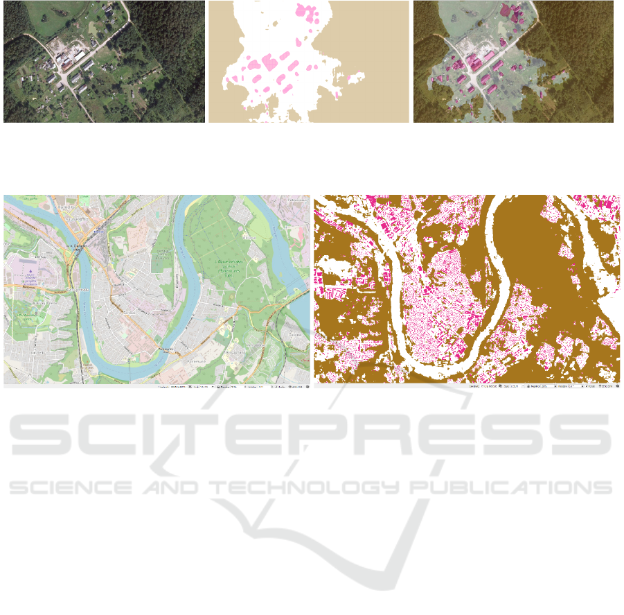
a)
b
)c)
Figure 8: a) Original ORTO10LT view; b-c) processed results and transparent original results with processed results of the
selected period (in this case, 2009-2010).
a
b
Figure 9: a) OSM data of Kaunas city centre; b) processed data of Kaunas city centre of the selected time period (in this case,
2009-2010).
On the finest level, each period has its own layer
which can be visualised using standard map software,
i.e. QGis, ArcGis, etc. Fig. 8-9 demonstrate the
results obtained with the model using the QGIS
software.
4 DISCUSSION AND
CONCLUSIONS
Object detection approaches are usually applied to
specific problems and small regions (Liu et al., 2020),
(Ye et al., 2019), (Wu et al., 2018), (Dornaika et al.,
2016), (Vakalopoulou et al., 2015), while on a
country level, only a limited amount of research has
been conducted (Al-Ruzouq et al., 2017), (Albert et
al., 2017), (Jean et al., 2016). Studies, which applied
object detection on a country level, were usually
focused on the final result rather than the process
itself. In this case, our publication fills in the missing
gap by providing a methodological approach of how
to prepare the training data and reduce the error
between the time series of remote sensing data of
different quality. Thus, the provided methodological
approach can be applied in different countries for
aerial or satellite images in order to determine the
urban growth patterns. Several issues were identified
when analysing the aerial images in a time series,
which were caused by the fact that in time, the
technical capabilities enable to obtain better quality
(i.e. before 2000, visual data for the same region was
available only in grey scale compared to the current
RBG of 16 bit depth) or valid external data to ensure
the ground truth dataset for model training is
unavailable altogether. In this work, transfer learning
technique has been applied for creating a machine
learning model. The initially pre-trained DeepLabv3
model with a ResNet50 backbone trained on the
ImageNet data has been selected. The model
adjustment was carried out in two steps. Firstly,
adjustment was performed on the OSM data with an
autogenerated coarse dataset and the final adjustment
for each period with the revised data has been applied
at the fine-tuning stage. In the dataset preparation
stage, it was demonstrated that the neural network
using a base dataset such as OSM is capable of
making segmentation on a country level; however,
expert input is necessary due to the differences in
mapping, use of the most recent ground truth data and
the assumption that there are not much changes in
GISTAM 2021 - 7th International Conference on Geographical Information Systems Theory, Applications and Management
22

data over the years. Moreover, normalisation of the
different quality images on spectrum and contrast
allows for creating segmented categorical maps of
different periods. It enables to analyse and interpret
the results on different levels, where both generalised
and granular data is available. The generalised results
could be used to detect exceptional patterns by using
a contour or heat map, while for the granular level
analysis, it is possible to review a map on a specific
location, so that the experts could better understand
and interpret the generalised results.
ACKNOWLEDGEMENT
This research was supported by the Research,
Development and Innovation Fund of Kaunas
University of Technology (project grant No.
PP91L/19).
REFERENCES
Al-Ruzouq, R., Hamad, K., Shanableh, A., & Khalil, M.
(2017). Infrastructure growth assessment of urban areas
based on multi-temporal satellite images and linear
features. Annals of GIS, 23(3), 183–201.
https://doi.org/10.1080/19475683.2017.1325935
Albert, A., Kaur, J., & Gonzalez, M. C. (2017). Using
convolutional networks and satellite imagery to identify
patterns in urban environments at a large scale.
Proceedings of the ACM SIGKDD International
Conference on Knowledge Discovery and Data Mining,
Part F1296, 1357–1366. https://doi.org/10.1145/
3097983.3098070
Celik, T. (2009). Unsupervised change detection in satellite
images using principal component analysis and κ-
means clustering. IEEE Geoscience and Remote
Sensing Letters, 6(4), 772–776. https://doi.org/10.1109/
LGRS.2009.2025059
Corbane, C., Syrris, V., Sabo, F., Pesaresi, M., Soille, P., &
Kemper, T. (2020). Convolutional Neural Networks for
Global Human Settlements Mapping from Sentinel-2
Satellite Imagery. ArXiv.
de Jong, K. L., & Sergeevna Bosman, A. (2019).
Unsupervised Change Detection in Satellite Images
Using Convolutional Neural Networks. 2019
International Joint Conference on Neural Networks
(IJCNN), July, 1–8. https://doi.org/10.1109/
ijcnn.2019.8851762
Donaldson, D., & Storeygard, A. (2016). The view from
above: Applications of satellite data in economics.
Journal of Economic Perspectives, 30(4), 171–198.
https://doi.org/10.1257/jep.30.4.171
Dornaika, F., Moujahid, A., El Merabet, Y., & Ruichek, Y.
(2016). Building detection from orthophotos using a
machine learning approach: An empirical study on
image segmentation and descriptors. Expert Systems
with Applications, 58, 130–142. https://doi.org/
10.1016/j.eswa.2016.03.024
Goyette, N., Jodoin, P.-M., Porikli, F., Konrad, J., &
Ishwar, P. (2012). A new change detection benchmark
dataset. IEEE Workshop on Change Detection
(CDW’12) at CVPR’12, 1–8.
Jean, N., Burke, M., Xie, M., Davis, W. M., Lobell, D. B.,
& Ermon, S. (2016). Combining satellite imagery and
machine learning to predict poverty. Science,
353(6301), 790–794. https://doi.org/10.1126/
science.aaf7894
Kanagamalliga, S., & Vasuki, S. (2018). Contour-based
object tracking in video scenes through optical flow and
gabor features. Optik, 157, 787–797. https://doi.org/
10.1016/j.ijleo.2017.11.181
Krupinski, M., Lewiński, S., & Malinowski, R. (2019). One
class SVM for building detection on Sentinel-2 images.
1117635(November 2019), 6. https://doi.org/10.1117/
12.2535547
Längkvist, M., Kiselev, A., Alirezaie, M., & Loutfi, A.
(2016). Classification and segmentation of satellite
orthoimagery using convolutional neural networks.
Remote Sensing, 8(4). https://doi.org/10.3390/
rs8040329
Liu, Y., Han, Z., Chen, C., DIng, L., & Liu, Y. (2020).
Eagle-Eyed Multitask CNNs for Aerial Image Retrieval
and Scene Classification. IEEE Transactions on
Geoscience and Remote Sensing, 58(9), 6699–6721.
https://doi.org/10.1109/TGRS.2020.2979011
Marmanis, D., Galliani, S., Schindler, K., Zurich, E.,
Marmanis, D., Wegner, J. D., Galliani, S., Schindler,
K., Datcu, M., & Stilla, U. (2016). Semantic
Segmentation Of Aerial Images With An Ensemble Of
CNNS 3D reconstruction and monitoring of
construction sites using LiDAR and photogrammetric
point clouds View project Earth Observation Image
Librarian (EOLib) View project SEMANTIC
SEGMENTATION O. III(July), 12–19. https://doi.org/
10.5194/isprsannals-III-3-473-2016
Nahhas, F. H., Shafri, H. Z. M., Sameen, M. I., Pradhan, B.,
& Mansor, S. (2018). Deep Learning Approach for
Building Detection Using LiDAR – Orthophoto Fusion.
2018.
Shermeyer, J., & Van Etten, A. (2019). The Effects of
Super-Resolution on Object Detection Performance in
Satellite Imagery. http://arxiv.org/abs/1812.04098
Suraj, P. K., Gupta, A., Sharma, M., Paul, S. B., &
Banerjee, S. (2018). On monitoring development
indicators using high resolution satellite images. 1–36.
http://arxiv.org/abs/1712.02282
Vakalopoulou, M., Karantzalos, K., Komodakis, N., &
Paragios, N. (2015). Building detection in very high
resolution multispectral data with deep learning
features. International Geoscience and Remote Sensing
Symposium (IGARSS), 2015-Novem, 1873–1876.
https://doi.org/10.1109/IGARSS.2015.7326158
Verbesselt, J., Hyndman, R., Newnham, G., & Culvenor, D.
(2010). Detecting trend and seasonal changes in
satellite image time series. Remote Sensing of
Deep Learning Application for Urban Change Detection from Aerial Images
23

Environment, 114(1), 106–115. https://doi.org/
10.1016/j.rse.2009.08.014
Verbesselt, J., Zeileis, A., & Herold, M. (2012). Near real-
time disturbance detection using satellite image time
series. Remote Sensing of Environment, 123, 98–108.
https://doi.org/10.1016/j.rse.2012.02.022
Wang, B., Tang, S., Xiao, J. Bin, Yan, Q. F., & Zhang, Y.
D. (2019). Detection and tracking based tubelet
generation for video object detection. Journal of Visual
Communication and Image Representation, 58, 102–
111. https://doi.org/10.1016/j.jvcir.2018.11.014
Wang, J., Song, J., Chen, M., & Yang, Z. (2015). Road
network extraction: a neural-dynamic framework based
on deep learning and a finite state machine.
International Journal of Remote Sensing, 36(12),
3144–3169. https://doi.org/10.1080/01431161.2015.
1054049
Witwit, W., Zhao, Y., Jenkins, K., & Zhao, Y. (2017).
Satellite image resolution enhancement using discrete
wavelet transform and new edge-directed interpolation.
Journal of Electronic Imaging, 26(2), 023014.
https://doi.org/10.1117/1.jei.26.2.023014
Wu, G., Shao, X., Guo, Z., Chen, Q., Yuan, W., Shi, X., Xu,
Y., & Shibasaki, R. (2018). Automatic building
segmentation of aerial imagery usingmulti-constraint
fully convolutional networks. Remote Sensing, 10(3),
1–18. https://doi.org/10.3390/rs10030407
Wurm, M., Stark, T., Zhu, X. X., Weigand, M., &
Taubenböck, H. (2019). Semantic segmentation of
slums in satellite images using transfer learning on fully
convolutional neural networks. ISPRS Journal of
Photogrammetry and Remote Sensing, 150(December
2018), 59–69. https://doi.org/10.1016/j.isprsjprs.
2019.02.006
Xie, M., Jean, N., Burke, M., Lobell, D., & Ermon, S.
(2016). Transfer learning from deep features for remote
sensing and poverty mapping. 30th AAAI Conference
on Artificial Intelligence, AAAI 2016, 3929–3935.
Ye, Z., Fu, Y., Gan, M., Deng, J., Comber, A., & Wang, K.
(2019). Building extraction from very high resolution
aerial imagery using joint attention deep neural
network. Remote Sensing, 11(24), 1–21.
https://doi.org/10.3390/rs11242970
GISTAM 2021 - 7th International Conference on Geographical Information Systems Theory, Applications and Management
24
