Malware Classiﬁcation with GMM-HMM Models

Jing Zhao

, Samanvitha Basole

and Mark Stamp

Department of Computer Science, San Jose State University, San Jose, California, U.S.A.

Keywords:

Hidden Markov Model, HMM, Gaussian Mixture Model, GMM-HMM, Malware.

Abstract:

Discrete hidden Markov models (HMM) are often applied to malware detection and classiﬁcation problems.

However, the continuous analog of discrete HMMs, that is, Gaussian mixture model-HMMs (GMM-HMM),

are rarely considered in the ﬁeld of cybersecurity. In this paper, we use GMM-HMMs for malware classiﬁ-

cation and we compare our results to those obtained using discrete HMMs. As features, we consider opcode

sequences and entropy-based sequences. For our opcode features, GMM-HMMs produce results that are

comparable to those obtained using discrete HMMs, whereas for our entropy-based features, GMM-HMMs

generally improve signiﬁcantly on the classiﬁcation results that we have achieved with discrete HMMs.

1 INTRODUCTION

Due to COVID-19, businesses and schools have

moved their work online and some consider the possi-

bility of going online permanently. This trend makes

cybersecurity more important than ever before.

Malicious software, or malware, is designed to

steal private information, delete sensitive data with-

out consent, or otherwise disrupt computer sys-

tems. The study of malware has been active for

decades (Milosevic, 2013). Malware detection and

classiﬁcation are fundamental research topics in mal-

ware. Traditionally, signature detection has been the

most prevalent method for detecting malware, but re-

cently, machine learning techniques have proven their

worth, especially for dealing with advanced types of

malware. Many machine learning approaches have

been applied to the malware problem, including hid-

den Markov models (HMM) (Stamp, 2018), k-nearest

neighbors (KNN) (Ben Abdel Ouahab et al., 2020),

support vector machines (SVM) (Kruczkowski and

Szynkiewicz, 2014), and a wide variety of neural net-

working and deep learning techniques (Kalash et al.,

2018).

Each machine learning technique has its own ad-

vantages and disadvantages. It is not the case that one

technique is best for all circumstances, since there are

many different types of malware and many different

features that can be considered. Thus, it is useful to

https://orcid.org/0000-0003-3182-4136

https://orcid.org/0000-0002-9806-3311

https://orcid.org/0000-0002-3803-8368

explore different techniques and algorithms in an ef-

fort to extend our knowledge base for effectively deal-

ing with malware. In this paper, we focus on Gaus-

sian mixture model-hidden Markov models (GMM-

HMMs), which can be viewed as the continuous ana-

log of the ever-popular discrete HMM.

Discrete HMMs are well known for their ability to

learn important statistical properties from a sequence

of observations. For a sequence of discrete observa-

tions, such as the letters that comprise a selection of

English text, we can train a discrete HMM to deter-

mine the parameters of the (discrete) probability dis-

tributions that underlie the training data. However,

some observation sequences are inherently continu-

ous, such as signals extracted from speech. In such

cases, a discrete HMM is not the ideal tool. While

we can discretize a continuous signal, there will be

some loss of information. As an alternative to dis-

cretization, we can attempt to model the continuous

probability density functions that underlie continuous

training data.

Gaussian mixture models (GMM) are probabil-

ity density functions that are represented by weighted

sums of Gaussian distributions (Reynolds, 2015). By

varying the number of Gaussian components and

the weight assigned to each, GMMs can effectively

model a wide variety of continuous probability dis-

tributions. It is possible to train HMMs to learn the

parameters of GMMs, and the resulting GMM-HMM

models are frequently used in speech recognition (Ra-

biner, 1989; Bansal et al., 2008), among many other

applications.

Zhao, J., Basole, S. and Stamp, M.

Malware Classiﬁcation with GMM-HMM Models.

DOI: 10.5220/0010409907530762

In Proceedings of the 7th International Conference on Information Systems Security and Privacy (ICISSP 2021), pages 753-762

ISBN: 978-989-758-491-6

753

In the ﬁeld of cybersecurity, GMMs have been

used, for example, as a clustering method for malware

classiﬁcation (Interrante-Grant and Kaeli, 2018).

However, to the best of our knowledge, GMM-HMMs

are not frequently considered in the context of mal-

ware detection or classiﬁcation. In this paper, we ap-

ply GMM-HMMs to the malware classiﬁcation prob-

lem, and we compare our results to discrete HMMs.

Our results indicate that GMM-HMMs applied to

continuous data can yield strong results in the mal-

ware domain.

The remainder of this paper is organized as fol-

lows. In Chapter 2, we discuss relevant related work.

Chapter 3 provides background on the various mod-

els considered, namely, GMMs, HMMs, and GMM-

HMMs, with the emphasis on the latter. Malware

classiﬁcation experiments and results based on dis-

crete features are discussed in Chapter 4. Since

GMM-HMMs are more suitable for continuous ob-

servations, in Chapter 4 we also present a set of mal-

ware classiﬁcation experiments based on continuous

entropy features. We conclude the paper and provide

possible directions for future work in Chapter 5.

2 RELATED WORK

A Gaussian mixture model (GMM) is a probability

density model (McLachlan and Peel, 2004) consist-

ing of a weighted sum of multiple Gaussian distribu-

tions. The advantage of a Gaussian mixture is that it

can accurately model a variety of probability distribu-

tions (Gao et al., 2020). That is, a GMM enables us to

model a much more general distribution, as compared

to a single Gaussian. Although the underlying distri-

bution may not be similar to a Guassian, the combi-

nation of several Gaussians yields a robust model (Al-

fakih et al., 2020). However, the more Gaussians that

comprise a model, the costly the calculation involving

the model.

One example of the use of GMMs is distribution

estimation of wave elevation in the ﬁeld of oceanogra-

phy (Gao et al., 2020). GMMs have also been used in

the ﬁelds of anomaly detection (Chen and Wu, 2019),

and signal mapping (Raitoharju et al., 2020). As an-

other example, in (Qiao et al., 2019), a GMM is used

as a classiﬁcation method to segment brain lesions. In

addition to distribution estimation, GMMs form the

basis for a clustering method in (Gallop, 2006).

As the name suggests, a discrete hidden Markov

model (HMM) includes a “hidden” Markov process

and a series of observations that are probabilistically

related to the hidden states. An HMM can be trained

based on an observation sequence, and the result-

ing model can be used to score other observation se-

quences. HMMs have found widespread use in signal

processing, and HMMs are particularly popular in the

area of speech recognition (Guoning Hu and DeLiang

Wang, 2004). Due to their robustness and the efﬁ-

ciency, HMMs are also widely used in medical ar-

eas, such as sepsis detection (Stanculescu et al., 2014)

and human brain studies based on functional mag-

netic resonance imaging (Dang et al., 2017). Motion

recognition is another area where HMMs play a vi-

tal role; speciﬁc examples include recognizing danc-

ing moves (Laraba and Tilmanne, 2016) and 3D ges-

tures (Truong and Zaharia, 2017).

Gaussian mixture model-HMMs (GMM-HMM)

are also widely used in classiﬁcation problems. Given

the ﬂexibility of GMMs, GMM-HMMs are pop-

ular for dealing with complex patterns underlying

sequences of observations. For example, Yao et

al. (Yao et al., 2020) use GMM-HMMs to clas-

sify network trafﬁc from different protocols. GMM-

HMMs have also been used in motion detection—

for complex poses, GMM-HMMs outperform dis-

crete HMMs (Zhang et al., 2020).

3 BACKGROUND

In this section, we ﬁrst introduce the learning tech-

niques used in this paper—speciﬁcally, we dis-

cuss Gaussian mixture models, HMMs, and GMM-

HMMs. We then discuss GMM-HMMs in somewhat

more detail, including various training and parameter

selection issues, and we provide an illustrative exam-

ple of GMM-HMM training.

3.1 Gaussian Mixture Models

As mentioned above, a GMM is a probabilistic model

that combines multiple Gaussian distributions. Math-

ematically, the probability density function of a GMM

is a weighted sum of M Gaussian probability density

functions. The formulation of a GMM can be written

as (Fraley and Raftery, 2002)

P(x |λ) =

∑

x=i

g(x |µ

, Σ

where x is a D-dimensional vector and ω

is the weight

assigned to the i

Gaussian component, with the mix-

ture weights summing to one. Here, µ

and Σ

are

the mean and the covariance matrix of the i

com-

ponent of the GMM, respectively. Each component

of a GMM is a multivariate Gaussian distribution of

ForSE 2021 - 5th International Workshop on FORmal methods for Security Engineering

754

the form

g(x |µ

, Σ

) =

(2π)

|Σ

−

(x−µ

)

−1

(x−µ

)

3.2 Discrete HMM

In this paper, we use the notation in Table 1 to de-

scribe a discrete HMM. This notation is essentially

the same as that given in (Stamp, 2018). An HMM,

which we denote as λ, is deﬁned by the matrices A, B,

and π, and hence we have λ = (A, B, π).

Table 1: Discrete HMM notation.

Notation Explanation

T Length of the observation sequence

O Observation sequence, O

, O

, . . . , O

T −1

N Number of states in the model

K Number of distinct observation symbols

Q Distinct states of the Markov process, q

, q

, . . . , q

N−1

V Observable symbols, assumed to be 0, 1, . . . , K − 1

π Initial state distribution, 1 × N

A State transition probabilities, N × N

B Observation probability matrix, N × K

We denote the elements in row i and column j of A

as a

i j

. The element a

i j

of the A matrix is given by

i j

= P(state q

at t +1 | state q

at t).

The (i, j) element of B is denoted in a slightly un-

usual form as b

( j). In a discrete HMM, row i of B

represents the (discrete) probability distribution of the

observation symbols when underlying Markov pro-

cess is in (hidden) state i. Speciﬁcally, each element

of B = {b

( j)} matrix is given by

( j) = P(observation j at t | state q

at t).

The HMM formulation can be used to is solve the

following three problems (Stamp, 2018).

1. Given an observation sequence O and a model λ

of the form λ = (π, A, B), calculate the probability

of the observation sequence. That is, we can score

an observation sequence against a given model.

2. Given a model λ = (π, A, B) and an observation

sequence O, ﬁnd the “best” state sequence, where

best is deﬁned to be the sequence that maximizes

the expected number of correct states. That is, we

can uncover the hidden state sequence.

3. Given an observation sequence O, determine a

model λ = (A, B, π) that maximizes P(O |λ). That

is, we can train a model for a given observation

sequence.

In this research, we are interested in problems 1 and 3.

Speciﬁcally, we train models, then we test the result-

ing models by scoring observation sequences. The

solution to problem 2 is of interest in various NLP

applications, for example. For the sake of brevity,

we omit the details of training and scoring with dis-

crete HMMs; see (Stamp, 2018) or (Rabiner, 1989)

for more information.

3.3 GMM-HMM

The structure of a GMM-HMM is similar to that of

a discrete HMM. However, in a GMM-HMM, the B

matrix is much different, since we are dealing with a

mixture of (continuous) Gaussian distributions, rather

than the discrete probability distributions a discrete

HMM. In a GMM-HMM, the probability of an ob-

servation at a given state is determined by a prob-

ability density function that is deﬁned by a GMM.

Speciﬁcally, the probability density function of obser-

vation O

when the model is in state i is given by

) =

∑

m=1

g(O

|µ

, Σ

), (1)

for i ∈ {1, 2, . . . , N} and t ∈ {0, 1, . . . , T − 1, where

∑

m=1

= 1 for i ∈ {1, 2, . . . , N}.

Here, M is the number of Gaussian mixtures com-

ponents, c

is the mixture coefﬁcient or the weight

of m

Gaussian mixture at state i, while µ

and Σ

are the mean vector and covariance matrix for the m

Gaussian mixture at state i. We can rewrite g in equa-

tion (1) as

g(O

|µ

, Σ

) =

(2π)

|Σ

−

−µ

)

−1

−µ

)

where D is the dimension of each observation. In a

GMM-HMM, the A and π matrices are the same as in

a discrete HMM.

The notation for a GMM-HMM is given in

Table 2. This is inherently more complex than a dis-

crete HMM, due to the presence of the M Gaussian

distributions. Note that a GMM-HMM is deﬁned by

the 5-tuple

λ = (A, π, c, µ, Σ).

Analogous to a discrete HMM, we can solve the same

three problems with a GMM-HMM. However, the

process used for training and scoring with a GMM-

HMM differ signiﬁcantly as compared to a discrete

HMM.

3.4 GMM-HMM Training and Scoring

To use a GMM-HMM to classify malware samples,

we need to train a model, then use the resulting model

Malware Classiﬁcation with GMM-HMM Models

755

Table 2: GMM-HMM notation.

Notation Explanation

T Length of the observation sequence

O Observation sequence, O

, O

, . . . , O

T −1

N Number of states in the model

M Number of Gaussian components

D Dimension of each observation

π Initial state distribution, 1 × N

A State transition matrix, N ×N

c Gaussian mixture weight at each state, N × M

µ Means of Gaussians at each state, N × M × D

Σ Covariance of Gaussian mixtures, N ×M × D × D

to score samples—see the discussion of problems 1

and 3 in Section 3.2, above. In this section, we discuss

scoring and training in the context of a GMM-HMM

in some detail. We begin with the simpler problem,

which is scoring.

3.4.1 GMM-HMM Scoring

Given a GMM-HMM, which is deﬁned by the 5-tuple

of matrices λ = (A, π, c, µ, Σ), and a sequence of ob-

servations O = {O

, O

, . . . , O

T −1

}, we want to deter-

mine P(O |λ). The forward algorithm, which is also

known as the α-pass, can be used to efﬁciently com-

pute P(O |λ).

Analogous to a discrete HMM as discussed

in (Stamp, 2018), in the α-pass of a GMM-HMM, we

deﬁne

(i) = P(O

, O

, . . . , O

, x

= q

|λ),

that is, α

(i) is the probability of the partial sequence

of observation up to time t, ending in state q

at time t.

The desired probability is given by

P(O |λ) =

N−1

∑

i=0

T −1

(i).

The α

(i) can be computed recursively as

(i) =



N−1

∑

j=0

t−1

(i)a



). (2)

At time t = 0, from the deﬁnition it is clear that we

have α

(i) = π

In a discrete HMM, b

) gives the probability of

observing O

at time t when the underlying Markov

process is in state i. In a GMM-HMM, however,

simply replacing b

) in (2) by the GMM pdf cor-

responds to a point value of a continuous distribu-

tion. To obtain the desired probability, as discussed

in (Nguyen, 2016), we must integrate over of a small

region around observation O

, that is, we compute

) =

+ε

−ε

|θ

)dO, (3)

where θ

consists of the parameters c

, µ

and Σ

of the

GMM, and ε is a (small) range parameter.

3.4.2 GMM-HMM Training

The forward algorithm or α-pass calculates the prob-

ability of observing the sequence from the beginning

up to time t. There is an analogous backwards pass

or β-pass that calculates the probability of the tail of

the sequence, that is, the sequence from t + 1 to the

end. In the β-pass, we deﬁne

(i) = P(O

t+1

, O

t+2

, . . . , O

T −1

= q

, λ).

The β

(i) can be compute recursively via

(i) =

N−1

∑

j=0

i j

)β

t+1

( j)

where we the initialization is β

T −1

(i) = 1, which fol-

lows from the deﬁnition.

In a discrete HMM, to re-estimate the state transi-

tions in the A matrix, we ﬁrst deﬁne

(i, j) = P(x

= q

, x

t+1

= q

|O, λ)

which is the probability of being in state q

at time t

and transiting to state q

at time t + 1. Using

the α-pass and the β-pass, we can efﬁciently com-

pute γ

(i, j); see (Stamp, 2018) for the details. The

sum of these “di-gamma” values with respect to the

transiting states gives the probability of the obser-

vation being in state q

at time t, which we deﬁne

as γ

(i). That is,

(i) =

∑

j=1

(i, j).

Thus, we can re-estimate the elements of the A matrix

in a discrete HMM as

i j

T −2

∑

t=0

(i, j)

T −2

∑

t=0

(i)

To train a GMM-HMM, we use an analogous strategy

as that used for the discrete HMM. The GMM-HMM

analog of the di-gamma form is

( j, k) = P(x

= q

|k, O, λ),

where t = 0, 1, . . . , T − 2, and j = 1, 2, . . . , N, and we

have k = 1, 2, . . . , M. Here, γ

( j, k) represents the

probability of being state q

at time t with respect

to the k

Gaussian mixture. According to (Rabiner,

1989), these γ

( j, k) are computed as

( j, k) =

( j)β

( j)

∑

j=1

( j)β

( j)

N(O

|µ

, Σ

)

∑

m=1

N(O

|µ

, Σ

)

ForSE 2021 - 5th International Workshop on FORmal methods for Security Engineering

756

where the α

( j) and β

( j) are deﬁned above, and c

is the weight of the k

Gaussian mixture component.

The re-estimates for the weights c

of the Gaus-

sian mixtures are given by

ˆc

T −1

∑

t=0

( j, k)

T −1

∑

t=0

∑

k=1

( j, k)

, (4)

for j = 1, 2, . . . , N and k = 1, 2, . . . , M; see (Juang,

1985) and (Rabiner, 1989) for additional details. The

numerator in (4) can be interpreted as the expected

number of transitions from state q

as determined by

the k

Gaussian mixture while the denominator can

viewed as the expected transitions from state q

given

by the M Gaussian mixtures. Accordingly, the re-

estimation for µ

and Σ

are of the form

ˆµ

T −1

∑

t=0

( j, k)O

T −1

∑

t=0

( j, k)

and

T −1

∑

t=0

( j, k)(O

− µ

)(O

− µ

)

T −1

∑

t=0

( j, k)

for i = 1, 2, . . . , N and k = 1, 2, . . . , M.

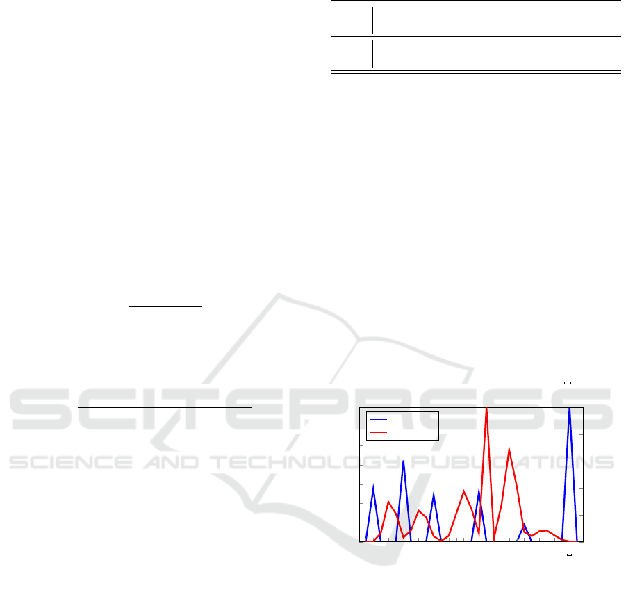
3.5 GMM-HMM Example

As an example to illustrate a GMM-HMM, we train

a model on English text, which is a classic exam-

ple for discrete HMMs (Cave and Neuwirth, 1980).

With N = 2 hidden states and M = 27 observation

symbols (corresponding the the 26 letters and word-

space), a discrete HMM trained on English text will

have one hidden state corresponding to consonants,

while the other hidden state corresponds to vowels.

That the model can make this key distinction is a good

example of learning, since a priori no information is

provided regarding the differences between the ob-

servations. We consider this same experiment using

a GMM-HMM to see how this model compares to a

discrete HMM.

The English training data is from the “Brown cor-

pus” (Brown Corpus of standard American English,

1961), and we convert all letters to lowercase and re-

move punctuation, numbers, and other special sym-

bols, leaving only 26 letters and word-spaces. For

our GMM-HMM training, we set N = 2, M = 6 (i.e.,

we have a mixture model consisting of 6 Gaussians)

Table 3: Mean of each Gaussian mixture in each state.

State

Gaussian

1 2 3 4 5 6

0 26.00 14.00 8.00 4.00 20.00 0.00

1 22.60 6.31 15.00 12.08 2.31 18.14

and T = 50000. The A matrix is N × N, π is 1 × N,

both of which are row stochastic, and initialized to ap-

proximately uniform. The parameter c represents the

weights of the mixture components and is initialized

with row stochastic values, also approximately uni-

form. We use the global mean value (i.e., the mean

of all observations) and global variance to initialize µ

and Σ. Note that each Gaussian is initialized with the

same mean and variance.

We train 100 of these GMM-HMM models, each

with different random initializations. As the obser-

vations are discrete symbols, the probability of each

observation in state i at time t is estimated by the prob-

ability density function. The best of the trained mod-

els clearly shows that the GMM-HMM technique is

able to successfully group the vowels into one state.

This can be seen from Figure 1. Note that in Figure 1,

word-space is represented by the symbol “ ”.

a b c d e f g h i j k l m n o p q r s t u v w x y z

Gaussian 1

0.00

0.05

0.10

0.15

0.20

0.25

Gaussian 2

Gaussian 1

Gaussian 2

Figure 1: English letter distributions in each state.

Figure 1 clearly shows that all vowels (and word

space) belong to the ﬁrst state. Table 3 lists the mean

value for each Gaussian mixture in the trained model.

The mean value of each Gaussian mixture component

corresponds to the encoded value of each observation

symbol.

In this example, since we know the number of

vowels beforehand, we have set the number of Gaus-

sian mixture components to 6 (i.e., 5 vowels and

word-space). In practice, we generally do not know

the true number of hidden states, in which case we

would need to experiment with different numbers of

Gaussians. In general, machine learning and deep

learning requires a signiﬁcant degree of experimen-

tation, so it is not surprising that we might need to

ﬁne tune our models.

Malware Classiﬁcation with GMM-HMM Models

757

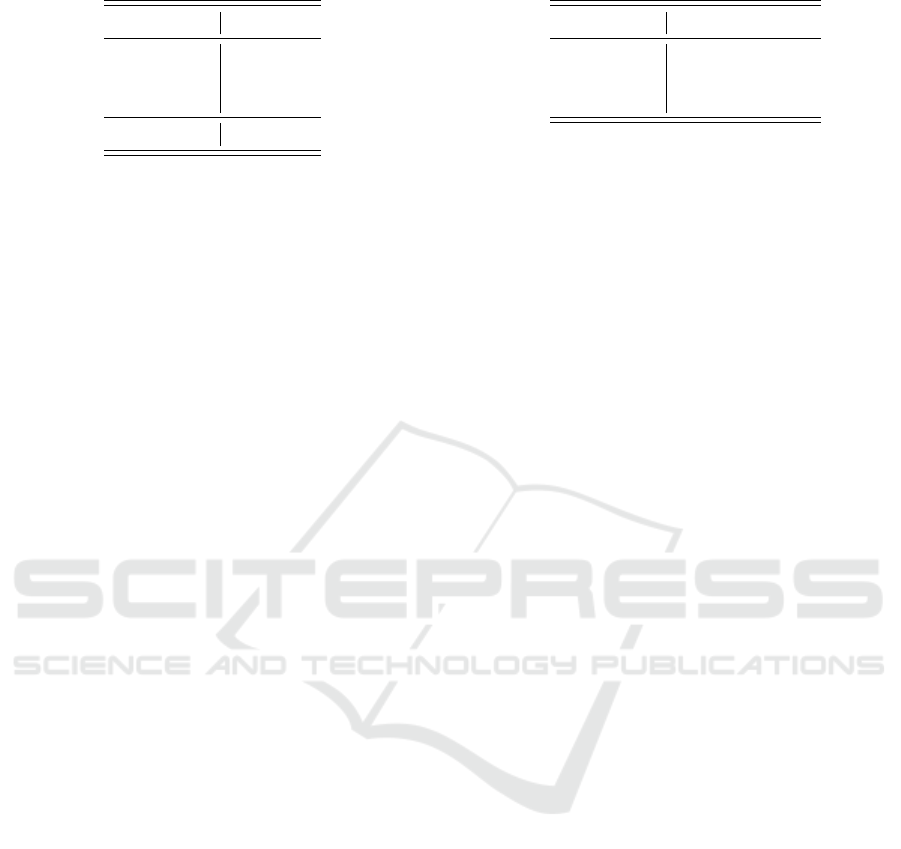
Table 4: Number of samples in each malware family.

Family Samples

Winwebsec 4360

Zeroaccess 2136

Zbot 1305

Total 7801

4 MALWARE EXPERIMENTS

In this section, we ﬁst introduce the dataset used in

our experiments, followed by two distinct sets of ex-

periments. In our ﬁrst set of experiments, we com-

pare the performance of discrete HMMs and GMM-

HMMs using opcode sequences as our features. In

our second set of experiments, we consider entropy

sequences, which serve to illustrate the strength of the

GMM-HMM technique.

4.1 Dataset

In all of our experiments, we consider three malware

families, namely, Winwebsec, Zbot, and Zeroaccess.

Winwebsec: is a type of Trojan horse in the Win-

dows operating system. It attempts to install ma-

licious programs by displaying fake links to bait

users (Winwebsec, 2017).

Zbot: is another type of Trojan that tries to steal user

information by attaching executable ﬁles to spam

email messages (Zbot, 2017).

Zeroaccess: also tries steal information, and it can

also cause other malicious actions, such as down-

loading malware or opening a backdoor (Neville

and Gibb, 2013).

Table 4 lists the number of samples of each malware

family in our dataset. These families are part of the

Malicia dataset (Nappa et al., 2015) and have been

used in numerous previous malware studies.

The samples of each malware family are split

into 80% for training and 20% for testing. We train

models on one malware family, and test the resulting

model separately against the other two families. Note

that each of these experiments is a binary classiﬁca-

tion problem.

We use the area under the ROC curve (AUC) as

our measure of success. The AUC can be interpreted

as the probability that a randomly selected positive

sample scores higher than a randomly selected nega-

tive sample (Bradley, 1997). We perform 5-fold cross

validation, and the average AUC from the 5 folds is

the numerical result that we use for comparison.

Table 5: Percentage of top 30 opcodes.

Family Top 30 opcodes

Winwebsec 96.9%

Zeroaccess 95.8%

Zbot 93.4%

4.2 Opcode Features

For our ﬁrst set of malware experiments, we compare

a discrete HMM and GMM-HMM using mnemonic

opcode sequences as features. To encode the input,

we disassemble each executable, then extract the op-

code sequence. We retain the most frequent 30 op-

codes with all remaining opcodes lumped together

into a single “other” category, giving us a total of 31

distinct observations. The percentage of opcodes that

are among the top 30 most frequent are listed in

Table 5.

For training, we limit the length of the observation

sequence to T = 100000, and for the discrete HMM,

we let N = 2. For the GMM-HMM, we we experi-

ment with the number of Gaussian mixtures ranging

from M = 2 to M = 5.

As mentioned above, we train a model with one

malware family and test with the other two mal-

ware families individually (i.e., in binary classiﬁca-

tion mode). To test each model’s performance, we use

one hundred samples from both families in the binary

classiﬁcation.

We initialize π and A to be approximately uniform,

as well as making them row stochastic. For each dis-

crete HMM, the B matrix is initialize similarly, while

for each GMM-HMM, the mean values and the co-

variance are initialized with the global mean value

and the global covariance of all training samples.

Figure 2 gives the average AUC (over the 5

folds) for models trained with discrete HMMs and the

GMM-HMMs with different values for m, the number

of Gaussians in the mixture. For most of the models,

the GMM-HMM is able to obtain comparable results

to the discrete HMM, and it does slightly outperform

a discrete HMM in some cases. but the improvement

is slight.

The results in Figure 2 indicate that for opcodes

sequences, GMM-HMMs perform comparably to dis-

crete HMMs. However, GMM-HMMs are more com-

plex and more challenging to train, and the additional

complexity does not appear to be warranted in this

case. But, this is not surprising, as opcode sequences

are inherently discrete features. To obtain a more

useful comparison, we next consider GMM-HMMs

trained on continuous features.

ForSE 2021 - 5th International Workshop on FORmal methods for Security Engineering

758

Test on Zeroaccess Test on Winwebsec

m = 2 m = 3 m = 4

m = 5

0.00

0.20

0.40

0.60

0.80

1.00

0.87

0.70

0.80

0.85

0.90

AUC

Discrete HMM

GMM-HMM

m = 2 m = 3 m = 4

m = 5

0.00

0.20

0.40

0.60

0.80

1.00

0.69

0.66

0.64

0.69

0.65

AUC

Discrete HMM

GMM-HMM

(a) Zbot models

Test on Zbot Test on Zeroaccess

m = 2 m = 3 m = 4

m = 5

0.00

0.20

0.40

0.60

0.80

1.00

0.72

0.57

0.61

0.65

0.66

AUC

Discrete HMM

GMM-HMM

m = 2 m = 3 m = 4

m = 5

0.00

0.20

0.40

0.60

0.80

1.00

0.83

0.68

0.59

0.73

0.83

AUC

Discrete HMM

GMM-HMM

(b) Winwebsec models

Test on Zbot Test on Winwebsec

m = 2 m = 3 m = 4

m = 5

0.00

0.20

0.40

0.60

0.80

1.00

0.71

0.68

0.72

0.66

0.64

AUC

Discrete HMM

GMM-HMM

m = 2 m = 3 m = 4

m = 5

0.00

0.20

0.40

0.60

0.80

1.00

0.61 0.61

0.65

0.61

0.57

AUC

Discrete HMM

GMM-HMM

Figure 2: Average AUC.

4.3 Entropy Features

GMM-HMMs are designed for continuous data, as

opposed to discrete features, such as opcodes. Thus

to take full advantage of the GMM-HMM technique,

we consider continuous entropy based features.

We use a similar feature-extraction method as

in (Baysa et al., 2013). Speciﬁcally, we consider the

raw bytes of an executable ﬁle, and we deﬁne a win-

dow size over which we compute the entropy. Then

we slide the window by a ﬁxed amount and repeat the

entropy calculation. Both the window size and the

slide amount are parameters that need to be tuned to

obtain optimal performance. In general, the slide will

be smaller than the window size to ensure no infor-

mation is lost.

Entropy is computed using Shannon’s well known

formula (Togneri and DeSilva, 2003)

E = −

∑

x∈W

p(x)log

p(x),

where W

is the i

window, and p(x) is the relative

frequency of the occurrence of the byte x within the

window W

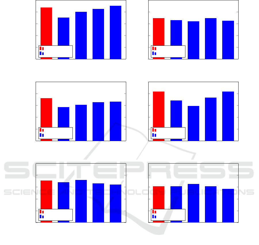
The entropy tends to be smoothed out with larger

window sizes. We want to select a window size sufﬁ-

ciently large so that we reduce noise, but not so large

as to lose useful information. Examples of entropy

plots for different parameters are given in Figure 3.

Malware Classiﬁcation with GMM-HMM Models

759

100

150

200

250

300

350

Window number

Entropy

(a) Window size = 512

0 200 400

600

800 1000 1200 1400

Window number

Entropy

(b) Window size = 128

Figure 3: Entropy plots.

Table 6: Window size and slide amount.

Window size 512 256 128

Slide 256 128 64

Based on the results in (Baysa et al., 2013), we use

half of the window size as the slide amount. To se-

lect the best values for the parameters, we conduct

experiments with the window and slide combinations

listed in Table 6. Also, as part of the parameter tuning

process, we selected ε in (3) to be 0.000001 for both

Zbot and Zeroaccess, while we ﬁnd 0.1 is optimal for

Winwebsec.

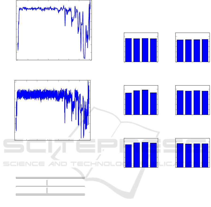
For models trained on Zbot, the results of our ex-

periments with the different window and slide size

pairings in Table 6 are given in Figure 4. We have

conducted analogous experiments for Winwebsec and

Zeroaccess; however for the sake of brevity, we have

omitted the corresponding bar graphs. Note that we

have experimented with the number of Gaussians in

our mixture ranging from m = 2 to m = 5. We see that

a window size of size 512 performs the worst, while

window sizes of size 256 and 128 give improved re-

sults, with size 128 being slightly better than 256. The

optimal number of Gaussians depends on the families

we are classifying.

Test on Winwebsec Test on Zeroaccess

m = 2 m = 3 m = 4

m = 5

0.00

0.20

0.40

0.60

0.80

1.00

0.92

0.91

0.92

0.91

Number of mixture components

AUC

m = 2 m = 3 m = 4

m = 5

0.00

0.20

0.40

0.60

0.80

1.00

0.86

0.87 0.87

0.88

Number of mixture components

AUC

(a) Window size = 512

Test on Winwebsec Test on Zeroaccess

m = 2 m = 3 m = 4

m = 5

0.00

0.20

0.40

0.60

0.80

1.00

0.85

0.94

0.97

0.86

Number of mixture components

AUC

m = 2 m = 3 m = 4

m = 5

0.00

0.20

0.40

0.60

0.80

1.00

0.94

0.92

0.94

0.92

Number of mixture components

AUC

(b) Window size = 256

Test on Winwebsec Test on Zeroaccess

m = 2 m = 3 m = 4

m = 5

0.00

0.20

0.40

0.60

0.80

1.00

0.89

0.97

0.98

0.95

Number of mixture components

AUC

m = 2 m = 3 m = 4

m = 5

0.00

0.20

0.40

0.60

0.80

1.00

0.94

0.92

0.93

0.92

Number of mixture components

AUC

Figure 4: Entropy vs window size for Zbot models.

In Table 7, we provide a direct comparison of discrete

HMMs trained on opcodes to GMM-HMM trained

on opcodes, as well as the best GMM-HMM mod-

els trained on (continuous) entropy sequences. In

every case, the entropy-trained GMM-HMM outper-

forms the corresponding opcode based models. It is

also worth noting that computing an entropy sequence

is more efﬁcient than extracting mnemonic opcodes.

While it is costlier to train a GMM-HMM, the scoring

cost is similar to that of a discrete HMM. Since train-

ing is one-time work, efﬁciency considerations also

favor the entropy-based GMM-HMM technique over

opcode-based HMMs.

From Table 7 we see that GMM-HMMs trained

on entropy perform dramatically better than discrete

HMMs, except in the two cases where models where

Zbot and Zeroaccess are involved. To gain fur-

ther insight into these anomalous case, we use the

ForSE 2021 - 5th International Workshop on FORmal methods for Security Engineering

760

Table 7: Comparison of discrete HMM and GMM-HMM.

Train Test

Opcode Opcode Entropy

HMM GMM-HMM GMM-HMM

Zbot Zeroaccess 0.87 0.90 0.94

Zbot Winwebsec 0.69 0.69 0.98

Zeroaccess Zbot 0.71 0.72 0.77

Zeroaccess Winwebsec 0.61 0.65 0.99

Winwebsec Zbot 0.72 0.66 1.00

Winwebsec Zeroaccess 0.83 0.83 1.00

Kullback–Leibler (KL) divergence (Joyce, 2011) to

compare the probability distributions deﬁned by of

our trained GMM-HMM models. The KL divergence

between two probability distributions is given by

KL(pk q) =

∞

−∞

p(x)log

p(x)

q(x)

, (5)

where p and q are probability density functions. Note

that the KL divergence in (5) is not symmetric, and

hence not a true distance measure. We compute a

symmetric version of the divergence for models M

and M

KL(M

, M

) =

KL(M

) + KL(M

)

. (6)

Using equation (6) we obtain the (symmetric) diver-

gence results in Table 8. We see that the Zbot and

Zeroaccess models are much closer in terms of KL

divergence, as compared to the other two pairs. Thus

we would expect GMM-HMM models to have more

difﬁculty distinguishing these two families from each

other, as compared to the models generated for the

other pairs of families.

Table 8: The KL divergence of different models.

Models KL divergence

Zbot, Zeroaccess 611.58

Zbot, Winwebsec 1594.05

Zeroaccess, Winwebsec 1524.39

Curiously, the models trained on Zbot and tested on

Zeroaccess perform well.

Hence, a relatively small

KL divergence does not rule out the possibility that

models can be useful, but intuitively, a large diver-

gence would seem to be an indicator of potentially

challenging cases. This issue requires further study.

It is worth noting that the opcode based models also

performed well in this case.

5 CONCLUSION AND FUTURE

WORK

In this paper, we have explored the usage of GMM-

HMMs for malware classiﬁcation, We compared

GMM-HMMs to discrete HMMs using opcode se-

quences, and we further experimented with entropy

sequences as features for GMM-HMMs. With the op-

code sequence features, we were able to obtained re-

sults with GMM-HMMs that are comparable to those

obtained using discrete HMMs, However, we expect

GMM-HMMs to perform best on features that are nat-

urally continuous, so we also experimented with byte-

based entropy sequences. In this latter set of exper-

iments, the GMM-HMM technique yielded stronger

results than the discrete HMM in all cases—and in

four of the six cases, the improvement was large. We

also directly compared the GMMs of our trained mod-

els using KL divergence, which seems to provide in-

sight into the most challenging cases.

For future work, more extensive experiments over

larger numbers of families with larger numbers of

samples per family would be valuable. True mul-

ticlass experiments based on GMM-HMM scores

would also be of interest. Further analysis of the KL

divergence of GMM-HMMs might provide useful in-

sights into these models.

REFERENCES

Alfakih, M., Keche, M., Benoudnine, H., and Meche, A.

(2020). Improved Gaussian mixture modeling for ac-

curate Wi-Fi based indoor localization systems. Phys-

ical Communication, 43.

Bansal, P., Kant, A., Kumar, S., Sharda, A., and Gupta,

S. (2008). Improved hybrid model of hmm/gmm for

speech recognition. In International Conference on

Intelligent Information and Engineering Systems, IN-

FOS 2008.

Baysa, D., Low, R., and Stamp, M. (2013). Structural en-

tropy and metamorphic malware. Journal of Com-

puter Virology and Hacking Techniques, 9(4):179–

192.

Ben Abdel Ouahab, I., Bouhorma, M., Boudhir, A. A.,

and El Aachak, L. (2020). Classiﬁcation of grayscale

malware images using the k-nearest neighbor algo-

rithm. In Ben Ahmed, M., Boudhir, A. A., Santos,

D., El Aroussi, M., and Karas,

I. R., editors, Innova-

tions in Smart Cities Applications, pages 1038–1050.

Springer, 3 edition.

Bradley, A. P. (1997). The use of the area under the

ROC curve in the evaluation of machine learning al-

gorithms. Pattern Recognition, 30(7):1145–1159.

Brown Corpus of standard American English (1961). The

Brown corpus of standard American English. http:

//www.cs.toronto.edu/

∼

gpenn/csc401/a1res.html.

Malware Classiﬁcation with GMM-HMM Models

761

Cave, R. L. and Neuwirth, L. P. (1980). Hidden Markov

models for English. In Ferguson, J. D., editor, Hidden

Markov Models for Speech. IDA-CCR.

Chen, Y. and Wu, W. (2019). Separation of geochemical

anomalies from the sample data of unknown distribu-

tion population using gaussian mixture model. Com-

puters & Geosciences, 125:9–18.

Dang, S., Chaudhury, S., Lall, B., and Roy, P. K. (2017).

Learning effective connectivity from fMRI using au-

toregressive hidden Markov model with missing data.

Journal of Neuroscience Methods, 278:87–100.

Fraley, C. and Raftery, A. E. (2002). Model-based clus-

tering, discriminant analysis, and density estima-

tion. Journal of the American Statistical Association,

97(458):611–631.

Gallop, J. (2006). Facies probability from mixture distribu-

tions with non-stationary impedance errors. In SEG

Technical Program Expanded Abstracts 2006, pages

1801–1805. Society of Exploration Geophysicists.

Gao, Z., Sun, Z., and Liang, S. (2020). Probability density

function for wave elevation based on Gaussian mix-

ture models. Ocean Engineering, 213.

Guoning Hu and DeLiang Wang (2004). Monaural speech

segregation based on pitch tracking and amplitude

modulation. IEEE Transactions on Neural Networks,

15(5):1135–1150.

Interrante-Grant, A. M. and Kaeli, D. (2018). Gaus-

sian mixture models for dynamic malware

clustering. https://coe.northeastern.edu/wp-

content/uploads/pdfs/coe/research/embark/4-

interrante-grant.alex ﬁnal.pdf.

Joyce, J. M. (2011). Kullback-Leibler divergence. In

Lovric, M., editor, International Encyclopedia of Sta-

tistical Science, pages 720–722. Springer.

Juang, B. (1985). Maximum-likelihood estimation for mix-

ture multivariate stochastic observations of Markov

chains. AT&T Technical Journal, 64(6):1235–1249.

Kalash, M., Rochan, M., Mohammed, N., Bruce, N. D. B.,

Wang, Y., and Iqbal, F. (2018). Malware classiﬁcation

with deep convolutional neural networks. In 2018 9th

IFIP International Conference on New Technologies,

Mobility and Security, NTMS, pages 1–5.

Kruczkowski, M. and Szynkiewicz, E. N. (2014). Sup-

port vector machine for malware analysis and classi-

ﬁcation. In 2014 IEEE/WIC/ACM International Joint

Conferences on Web Intelligence and Intelligent Agent

Technologies, WI-IAT ’14, pages 415–420.

Laraba, S. and Tilmanne, J. (2016). Dance performance

evaluation using hidden Markov models. Computer

Animation and Virtual Worlds, 27(3-4):321–329.

McLachlan, G. and Peel, D. (2004). Finite Mixture Models.

Wiley.

Milosevic, N. (2013). History of malware. https://arxiv.org/

abs/1302.5392.

Nappa, A., Raﬁque, M. Z., and Caballero, J. (2015).

The MALICIA dataset: Identiﬁcation and analysis of

drive-by download operations. International Journal

of Information Security, 14(1):15–33.

Neville, A. and Gibb, R. (2013). ZeroAccess Indepth. https:

//docs.broadcom.com/doc/zeroaccess-indepth-13-en.

Nguyen, L. (2016). Continuous observation hidden Markov

model. Revista Kasmera, 44(6):65–149.

Qiao, J., Cai, X., Xiao, Q., Chen, Z., Kulkarni, P., Ferris,

C., Kamarthi, S., and Sridhar, S. (2019). Data on MRI

brain lesion segmentation using k-means and Gaus-

sian mixture model-expectation maximization. Data

in Brief, 27.

Rabiner, L. R. (1989). A tutorial on hidden Markov models

and selected applications in speech recognition. Pro-

ceedings of the IEEE, 77(2):257–286.

Raitoharju, M., Garc

ıa-Fern

andez, A., Hostettler, R., Pich

R., and S

arkk

a, S. (2020). Gaussian mixture models

for signal mapping and positioning. Signal Process-

ing, 168:107330.

Reynolds, D. (2015). Gaussian mixture models. In Li, S. Z.

and Jain, A. K., editors, Encyclopedia of Biometrics,

pages 827–832. Springer.

Stamp, M. (2018). A revealing introduction to hid-

den Markov models. https://www.cs.sjsu.edu/

∼

stamp/

RUA/HMM.pdf.

Stanculescu, I., Williams, C. K. I., and Freer, Y. (2014).

Autoregressive hidden Markov models for the early

detection of neonatal sepsis. IEEE Journal of Biomed-

ical and Health Informatics, 18(5):1560–1570.

Togneri, R. and DeSilva, C. J. S. (2003). Fundamentals of

Information Theory and Coding Design. CRC Press.

Truong, A. and Zaharia, T. (2017). Laban movement analy-

sis and hidden Markov models for dynamic 3D ges-

ture recognition. EURASIP Journal on Image and

Video Processing, 2017.

Winwebsec (2017). Win32/winwebsec threat descrip-

tion - Microsoft security intelligence. https:

//www.microsoft.com/en-us/wdsi/threats/malware-

encyclopedia-description?Name=Win32/Winwebsec.

Yao, Z., Ge, J., Wu, Y., Lin, X., He, R., and Ma, Y.

(2020). Encrypted trafﬁc classiﬁcation based on

Gaussian mixture models and hidden Markov models.

Journal of Network and Computer Applications, 166.

Zbot (2017). Pws:win32/zbot threat description - Microsoft

security intelligence. https://www.microsoft.com/en-

us/wdsi/threats/malware-encyclopedia-description?

Name=PWS%3AWin32%2FZbot.

Zhang, F., Han, S., Gao, H., and Wang, T. (2020). A Gaus-

sian mixture based hidden Markov model for motion

recognition with 3D vision device. Computers & Elec-

trical Engineering, 83.

ForSE 2021 - 5th International Workshop on FORmal methods for Security Engineering

762