ECGraph: A Complex Networks Tool to Classify Critical Points

of Ecological Corridors

Gianni Fenu

and Enrico Podda

Department of Computer Science, University of Cagliari, Via Ospedale 72, 09124 Cagliari, Italy

Keywords:

Complex Networks, Ecological Networks, Ecological Corridors, Connectivity, Graph Analytics.

Abstract:

The analysis of large amounts of information and its representation in a simple model has always been one

of the main purposes of computer science. The ﬁeld of territorial study is an excellent example to observe

the complexity of the process, from the basic search for information through simple but expensive geometric

calculations to the connection that the information itself has concerning the rest of the territory. The study of

the natural areas identiﬁed by the European project Natura 2000 and their interconnection through the use of

ecological corridors is an example of how difﬁcult it can be to deﬁne, study and represent a complex problem.

In order to simplify the mentioned tasks, allowing specialists to consult valuable data, the paper exposes how

ECGraph works. This open source software allows extracting important information from any corridor related

to areas of the Natura 2000 project, and can potentially be generalized to any similar case.

1 INTRODUCTION

The delineation of the areas from the Natura 2000

project (Evans, 2012) (Ostermann, 1998) has been

an enormous improvement in the management and

preservation of European ﬂora and fauna (Urban and

Keitt, 2001) (Fenu and Pau, 2015). Natura 2000’s

main purpose is to protect the biodiversity of indige-

nous living beings on European soil, without however

precluding the already developed and massive human

infrastructures. Deﬁning and standardizing protected

areas in which plants and animals can live has allowed

the process of their possible extinction to slow down.

However, it is not enough, as it is trivial to note that

without sufﬁcient biodiversity an ecosystem cannot

thrive nor survive for long.

To help solving this pressing problem, studies

have led to the theorization of a valuable tool, the eco-

logical corridor.

Ecological corridors (Jongman, 1995) (Gill Jr

et al., 2009) have been designed to connect protected

areas through patches of land selected to satisfy spe-

ciﬁc walkability standards, allowing to emulate a path

for migration of species. If research progresses in

the standardization and implementation of ecological

corridors, it could allow autonomous sustainability of

https://orcid.org/0000-0003-4668-2476

https://orcid.org/0000-0001-5635-6610

the species that the Natura 2000 project seeks to pre-

serve. Nonetheless, design and manage such a net-

work would be all but easy.

Considering the territory as a Complex Network

could help to keep track of dangerous patches and pre-

vent possible events that may threaten the territory or

endanger the possibility to walk through the ecologi-

cal corridor (Bodini and Cossu, 2010). Complex Net-

works can in fact help to make useful considerations

on the state of a corridor and allow to read the confor-

mation of the territory in a more efﬁcient and precise

way. The most serious threat that can undermine the

usefulness of an ecological corridor would be its im-

practicability. A cut node (Fenu and Pau, 2018) can

indeed bring to that outcome.

To understand the central role in the research of

cut nodes it is necessary to imagine the ecological

corridor as a graph, where the patches correspond to

the nodes and the edges represent the adjacencies be-

tween neighbor patches. A cut node is a peculiar node

that if removed disconnects part of the nodes from

the graph, actually creating distinct and unconnected

subgraphs. As has already been fully explained in

previous studies (Fenu and Pau, 2018), not all cut

nodes preclude the possibility to walk through the

corridor, but some could represent a threat. Similar

considerations could also be made for the virtual cut

nodes (Fenu and Podda, 2020), which are different

from cut nodes. In fact, virtual cut nodes are formed

Fenu, G. and Podda, E.

ECGraph: A Complex Networks Tool to Classify Critical Points of Ecological Corridors.

DOI: 10.5220/0010388800470054

In Proceedings of the 6th International Conference on Complexity, Future Information Systems and Risk (COMPLEXIS 2021), pages 47-54

ISBN: 978-989-758-505-0

by a set of nodes which are not capable of breaking

the graph apart if taken individually. Up to this date

there is no open source code that has implemented a

way to detect cut nodes or virtual cut nodes clearly

and efﬁciently, even though some logic has been the-

orized.

Tools such as QGIS (Team et al., 2015) (Jenson

and Domingue, 1988) and its libraries are extremely

valid for the study and standardization of landscape.

QGIS provides a valid representation of raster and

vector maps and is able to query the attributes of the

layers so that useful information is displayed. The

tool also allows to run scripts developed in Python 3

in a console integrated with the program, but this can

quickly become limiting for our purposes.

ECGraph, the software described in this paper, is

proposed as a tool to identify critical points of the

network, such as cut nodes and virtual cut nodes.

Furthermore, the software also saves in the output

additional information that allows both to have an

overview of the network and to focus on the proper-

ties of the node (patch) in relation to the network it-

self. We decided to develop ECGraph with JavaScript

to be easily integrable by npm (Tilkov and Vinoski,

2010), to simplify future integration in projects with

a graphical interface that can offer features difﬁcult to

implement on QGIS at the moment. The paper will

also present the ECGraph output obtained from the

ecological corridor designed in previous studies (Can-

nas and Zoppi, 2017). The covered area refers to the

metropolitan area of Cagliari, an Italian municipality

located in the south of the island of Sardinia, of which

it is capital.

2 HOW ECGraph WORKS

The software, available on GitHub

, shows the algo-

rithm. Given as input an ecological corridor and the

areas it connects, ECGrapgh produces an output co-

incident to the same ecological corridor, but provided

with additional properties.

In the README of the repository, there is also a

link to download the input area. These areas are the

ones distributed by the Natura 2000 project, but ready

to run with the code. Information on how to use the

code and on the allowed commands is also shown in

the README.

It is important to point out that the steps described

below must be performed in the exact order they will

be presented. This will prevent the algorithm from

unnecessary and very time-consuming computations.

https://github.com/epilurzu/ecgraph

Furthermore, it assures to return values that would not

be correct otherwise. It should also be speciﬁed that

the main role of the software is to act as a valuable

tool for reading the complex relationships shown in

the analyzed network, and its main task is to verify

and give information regarding the conditions of the

network.

2.1 TopoJSON and Connected

Components

First of all, we determined that the best data structure

to use for the algorithm is TopoJSON

. The TopoJ-

SON format, being an extension of GeoJSON (But-

ler et al., 2016) that encodes topology, allows saving

data more efﬁciently than the latter. This is possible

because it simpliﬁes the data by saving the informa-

tion of the arcs that are part of the polygon perimeters

stored in the layer. By saving the geographic data in

this way, redundancy is avoided.

Unless the TopoJSON format is not only com-

posed of polygons with proprietary arcs as in the case

of an archipelago, it offers a reduction of 80% or more

in space without any need for simpliﬁcation. It is

also signiﬁcantly smaller than a shapeﬁle, and also

possesses all the readability properties of the JSON

ﬁles (Severance, 2012).

For these reasons, we decide to use this format as

an input for corridors and areas, and as an output for

the corridor improved with obtained data.

Among the many other beneﬁts it possesses, we

can take advantage of its neighbors function. The

TopoJSON format makes it especially easy to ﬁnd

neighbor nodes starting from a node, as neighbors

share an arc with the node. By recursively following

neighbors, we can deﬁne which is the connected and

integrated component (Fenu and Pau, 2018) (Fenu

and Nitti, 2011) in linear time. The efﬁciency in

developing a connected component and its immedi-

ate reading remain key points in the analysis of com-

plex networks in all ﬁelds in which it is applied (Orda

et al., 2019).

For the operations we are going to perform, the

connected component is the basis to start from. It

represents a set of nodes that can be reached through

adjacent nodes. From this deﬁnition, it is simple to

deduce that only an alteration of these nodes can en-

danger their structure, and nothing else. However, it

is necessary to pay attention to a peculiarity.

In fact, as software development has shown, and

as it can be deduced from the properties of the Topo-

JSON format, neighboring nodes that share a single

https://github.com/topojson/topojson-speciﬁcation/

blob/master/README.md

COMPLEXIS 2021 - 6th International Conference on Complexity, Future Information Systems and Risk

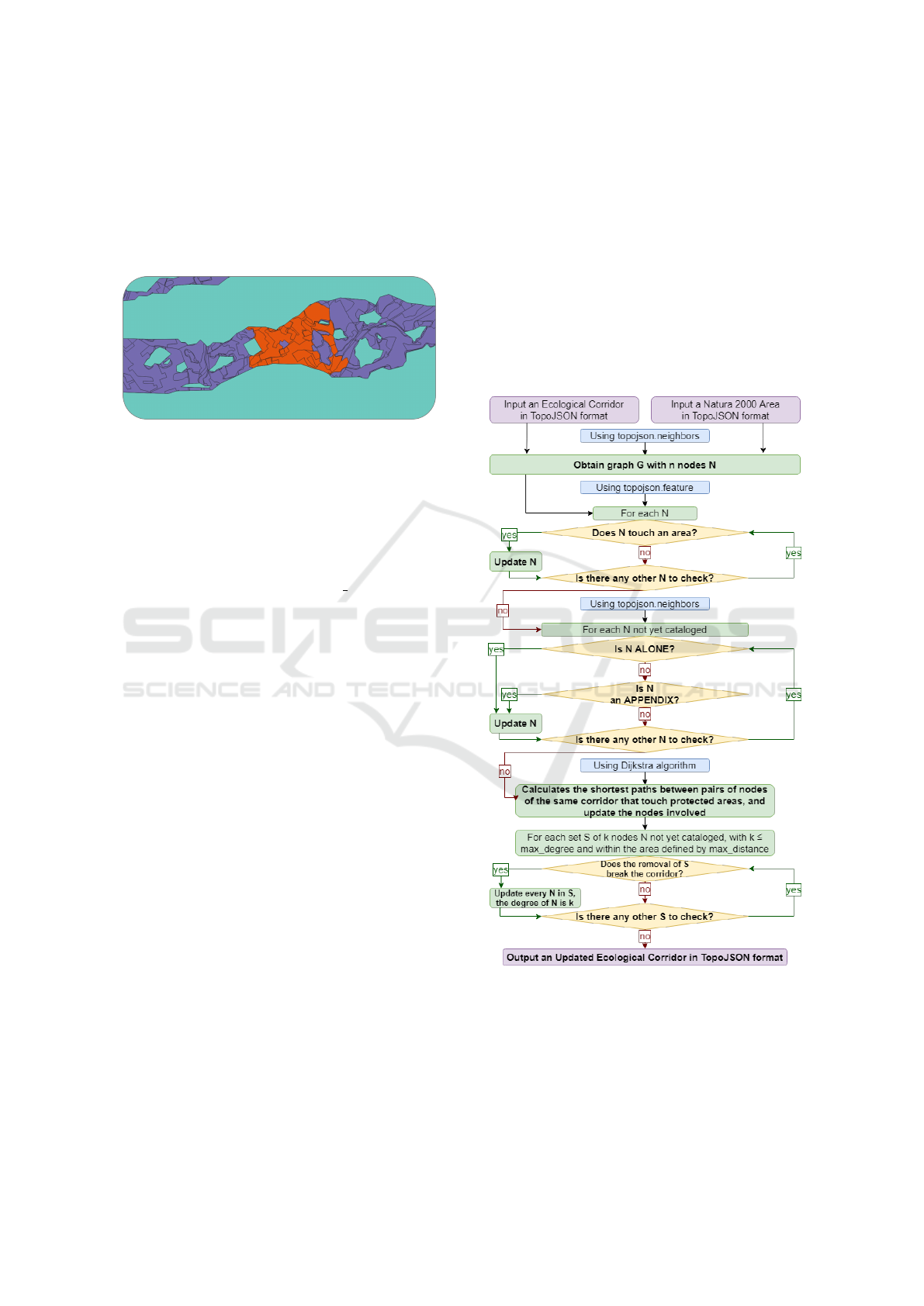
Figure 1: On top an example of a corridor in purple, at the

bottom a zoom of the same corridor. There are some indi-

vidual patches highlighted in orange. These are not consid-

ered to be a part of the main connected component because

they do not share a common arch with their neighbors.

point like the one shown in Figure 1 are not consid-

ered neighbors at all.

Although in a practical case this difference might

seem negligible, it represents a substantial difference

for the algorithm. Furthermore, depending on the an-

imal species whose migration is examined, it may be

unreasonable to consider that they could be channeled

into such a bottleneck.

2.2 Patches with Neighbor Areas

Among the most important patches, we certainly ﬁnd

those bordering protected areas (Ostermann, 1998).

They represent the source and sink nodes in the pas-

sage between the areas. In case of migration, these

essential nodes are certainly traversed. However, to

identify these patches we cannot use the neighbor

method used in the subsection 2.1, because they are

not part of the same layer. In fact, it is not even cer-

tain that the patches lie on the perimeter of the area,

the two of them could also overlap. A different ap-

proach is needed, which requires more computational

and time resources, but is equally effective.

First of all, it is necessary to momentarily convert

the corridor and area ﬁles into GeoJSON via function

topojson.feature. This allows access to the real co-

ordinates representing the individual polygons and to

perform simple intersection operations. We choose to

use the Turfjs

library for this task. Identifying bor-

dering areas and patches at this point is a problem of

https://turfjs.org/

quadratic complexity, as two nested for are needed to

iterate the various combinations. It is not even pos-

sible to stop the cycle for a speciﬁc patch once the

intersection with a protected area has been identiﬁed,

as there are areas themselves that intersect other areas,

potentially making a patch bordering both.

To further simplify the calculation is necessary to

ﬁlter the protected areas ﬁrst. Doing so, ECGraph

obtains only those areas that are touched by at least

one patch and avoids unnecessary operations. This is

done by deﬁning a bounding box of the corridor and

ﬁltering the areas that intersect with it. At this point,

the search operation is greatly simpliﬁed but is still

expensive enough to demand at least seconds in the

best-case scenario.

As a preliminary operation to the steps described

in the subsection, we decided to simplify the two in-

put layers with the topojson.presimplify function, so

that the number of points that deﬁne the polygons

could be decreased. The accuracy of the resulting lay-

ers can be chosen by the user. It must be the object of

particular care because if set poorly it could remove

entire areas, or not ﬁnd intersections that instead exist.

At the end of this phase, the variable vcn degree

of the identiﬁed nodes will be set with a particular

code deﬁne as NEIGHBOR OF AREA that will dis-

tinguish them as bordering a protected area.

2.3 Isolated Patches and Appendices

As mentioned in subsection 2.1, some connected

components may be composed of single nodes due to

the conformation of the territory and the speciﬁcs of

the TopoJSON format. In subsection 2.2, on the other

hand, it was found that the prior removal of elements

that are not useful for the computation can make a

huge difference, especially in terms of time.

This subsection lays the foundations to avoid un-

necessary operations in following iterations, and with

a linear computational cost. In fact, from this point

on, the algorithm will work only on nodes that do not

have vcn degree initialized, except in some cases for

similar degrees.

For the ﬁrst skimming, the software removes the

nodes without neighbors, i.e. completely isolated.

These, by deﬁnition, could never be cut nodes, but

they still do not have any use in traversing the cor-

ridor. If not cataloged they would only add worth-

less computations later on. Once identiﬁed, their

vcn

degree can be set to ALONE.

There are, however, another category of nodes that

are not useful for crossing the corridor, those who

necessarily have to cross the same node twice in or-

der not to get stuck. An example of these nodes is

ECGraph: A Complex Networks Tool to Classify Critical Points of Ecological Corridors

the enclaves (Fenu and Pau, 2018), nodes surrounded

by other nodes, and not accessible by any other route.

However, they are not the only ones that fall within

the deﬁnition. Generalizing, we could deﬁne ap-

pendix nodes all those that have among their neigh-

bors some nodes that are appendix and at most one

neighbor that is not, as shown in the Figure 2.

Figure 2: Some examples of appendices, highlighted in or-

ange, through different corridors, colored in purple.

Once identiﬁed, it is possible to set their vcn degree

to APPENDIX. This further simpliﬁcation can make

a signiﬁcant difference in terms of time depending

on the conformation of the corridor and does not re-

quire differentiation of the enclaves from the other ap-

pendix nodes, as they all have the same property.

It is however necessary to specify that some nodes

cataloged as appendices could also be cut nodes, but

if removed they could not jeopardize the ability to

walk through the ecological corridor. Once an ap-

pendix node has been eliminated, the excluded sub-

graph would have no access to natural areas, being

therefore negligible.

2.4 Shortest Path

Once the least used nodes have been removed, it is

now necessary to score the nodes based on their fre-

quency of use. We choose to use the Dijkstra algo-

rithm (Dijkstra et al., 1959) to search for the short-

est path in order to identify which nodes are being

traveled and how often. First of all, it is necessary to

identify each pair of nodes that would start and arrive

at different natural areas and who join the same con-

nected component. This step is possible thanks to the

information obtained from the subsection 2.2.

Once the various start and end nodes are found,

the sp score variable of the nodes belonging to the

shortest path has to increase by one. Once ﬁnished in-

creasing all the nodes of the various shortest path cal-

culated in the connected component, is now required

to normalize the data by dividing the same variable by

the total number of shortest path calculated.

Doing so, the value can vary from 0, a node never

traveled, to 1, a node traveled by every single short-

est path. In a nutshell, is possible to see the sp score

variable as a betweenness centrality of the network

calculate for nodes source and sink that are adjacent

to protected areas. As a cost variable for the choice of

the least expensive node in Dijkstra’s algorithm, we

choose to use the distance between centroids of the

nodes, so that the algorithm prefers a greater number

of nodes to travel if this means saving time to travel

them in a practical case. The time complexity of this

algorithm is k O(n

) with k equal to the number of

source-sink combinations.

2.5 Cut Nodes and Virtual Cut Nodes

Finally, it is possible to give a classiﬁcation of the

nodes that can affect the possibility to walk through

the connected components if removed. As already

explained in other papers (Fenu and Pau, 2018) a cut

node can be deﬁned as a node that, if removed from

the component, divides it into more subcomponents

not connected. Similarly, virtual cut nodes (Fenu and

Podda, 2020) are groups of nodes that if removed si-

multaneously cause the same consequences as the re-

moval of a cut node.

To identify a cut node among the nodes still with-

out vcn

degree, the algorithm creates a connected

subcomponent starting from a neighbor of the node

under analysis, from which it recursively runs through

the neighbors to create the network as seen in the sub-

section 2.1. However, the subcomponent cannot ex-

pand if one of the neighbors corresponds to the con-

sidered node, in order to simulate its removal. At the

end of the creation of the subcomponent, if it is com-

posed of a number of nodes lower than the original

component -1, we will have the evidence that the cho-

sen node is actually a cut node.

The algorithm can be generalized so that it can

calculate virtual cut nodes of any degree, but there

are some reﬂections to be made. It is necessary to test

if groups of nodes, currently uncataloged, of size n,

with n corresponding to the degree of the possible vir-

tual cut node, are indeed virtual cut nodes. However,

testing each individual combination would be compu-

tationally expensive. Although it has been shown that

virtual cut nodes can have child nodes even at multi-

COMPLEXIS 2021 - 6th International Conference on Complexity, Future Information Systems and Risk

ple nodes apart (Fenu and Podda, 2020), it has been

found that this is not a frequent event. To simplify the

computation, we decide to impose a maximum limit

of steps from the father node in which to search for

candidates neighbors to join the possible virtual cut

node, as shown in Figure 3.

Figure 3: The heart-shaped parent patch in the center is

surrounded by orange highlighted patches. The selected

patches correspond to all the neighbors in the corridor that

are no more than 3 steps from the parent node.

Doing so, in the worst case, the unnecessary iterations

would be limited to that set of neighbors. Always for

time and computation savings reasons, we also decide

not to keep track of founded virtual cut nodes, but in-

stead to mark the corresponding vcn degree or every

single node belonging to the virtual cut node of de-

gree n found. In fact, each of those nodes is sure to

be part of at least one virtual cut node, that is the one

found. Doing so, for every virtual cut node of degree

n, n nodes are set, and numerous cycles are avoided.

As in the cut node search, once created a subcompo-

nent that propagates avoiding the points of the virtual

cut node, if this is less than the size of the component

- n, then a new virtual cut node has been identiﬁed.

At the end of the iteration of this part of the algo-

rithm, the search for the various virtual cut node con-

taining a father node can be easily found by repeat-

ing a similar algorithm only on the identiﬁed nodes of

the father’s degree. As mentioned above, running the

algorithm in order of increasing degree is necessary.

It not only decreases the number of cycles needed to

calculate higher degrees by removing the lower ones

but also prevents recognizing erroneously some vir-

tual cut node that could break the graph with a subset

of itself. That would result in a virtual cut node with

a lower degree. This information makes a huge dif-

ference as if a virtual cut node is of a lower degree

it is much more threatening for the network structure.

The ﬁnal user can set at will the maximum distance

in which to search for virtual cut nodes and the maxi-

mum degree wanted.

To calculate the time complexity it is necessary to

consider how many times it is required to build the

check subgraph, with linear time complexity. In the

case of cut nodes, it is simply one. In the case of

virtual cut nodes, it is necessary to take into consider-

ation the set k of possible child nodes that are distant

from the father node the number of steps chosen or

less. In the worst case scenario, the check subgraph

has to be estimated for each n-1 element subset of the

set k, with n being the current virtual cut node degree.

2.6 Time and Score

The Figure 4 shows with a ﬂow chart the main pro-

gresses of the program illustrated in this paper.

Figure 4: A simple ﬂowchart showing the main points of

ECGraph. The inputs and outputs are highlighted in pur-

ple, some functions used by the program in blue, and the

operations it performs in green and yellow.

As seen in previous subsections, ECGraph allows the

user to specify the accuracy wanted to ﬁnd intersec-

tions between corridors and areas, the maximum de-

gree desired in the research of a virtual cut node and

ECGraph: A Complex Networks Tool to Classify Critical Points of Ecological Corridors

the maximum distance where to search for it. This

parameters let the user obtain higher precision of the

output data. This, requiring a greater number of iter-

ations, leads to a consequential increase in execution

time.

The algorithm has been tested giving different ac-

curacy as input to topojson.presimplify. These, by

inﬂuencing the precision of the polygons examined

in the calculation of the intersections seen in subsec-

tion 2.2, will directly affect the search times of the

protected areas adjacent to the corridor and neighbor

to speciﬁc patches. In a nutshell, greater accuracy

in topojson.presimplify should avoid ﬁnding corridor

patches neighbor of protected areas that result in false

positives or false negatives.

As for the maximum degree of virtual cut node to

be searched, we set it to four, while keeping the exe-

cution times of the single degree separate. What can

increase computation times in this case is the exten-

sion of the nodes to be tested as possible children, by

setting a greater maximum distance to choose from as

seen in the subsection 2.5

The results obtained by running the program on

the same input corridor (Cannas and Zoppi, 2017) is

show in Tables 1 and 2 and represented in the Fig-

ure 5. The computer used to run the code is equipped

with an AMD A10 7850k processor and two 4GB

DDR3 1866MHz RAM. The program runs on a single

thread.

The clearest difference lies in the search for nodes

connected with natural areas. As shown in Figure 5,

the algorithm executed with higher accuracy recog-

nized a relatively small protected area, and has conse-

quently found all patches that intersect it. In terms of

search time, the difference is important and as a result,

the inclusion of three more areas occurred. Those

same areas would have been lost in the simpliﬁcation,

with the consequent reduction in terms of time seen

in Table 1.

This consequently increases the number of short-

est paths requested and leads to an increase in time

in that section of the algorithm as well. As far as

cut nodes and virtual cut nodes are concerned, these

have been partly converted into nodes bordering ar-

eas, but in addition to this, they have not shown dras-

tic increases related to a larger area in their search, as

shown in Table 2.

For a clearer combined representation of the main

values obtained, a new variable containing a normal-

ization of vcn degree and sp score has been imple-

mented. It can be calculated a normalized vcn score

from nodes with vcn degree ≥ 1 by dividing 1 by

vcn degree, so that the variable can only have val-

ues from 0 to 1. Multiplying then the vcn score with

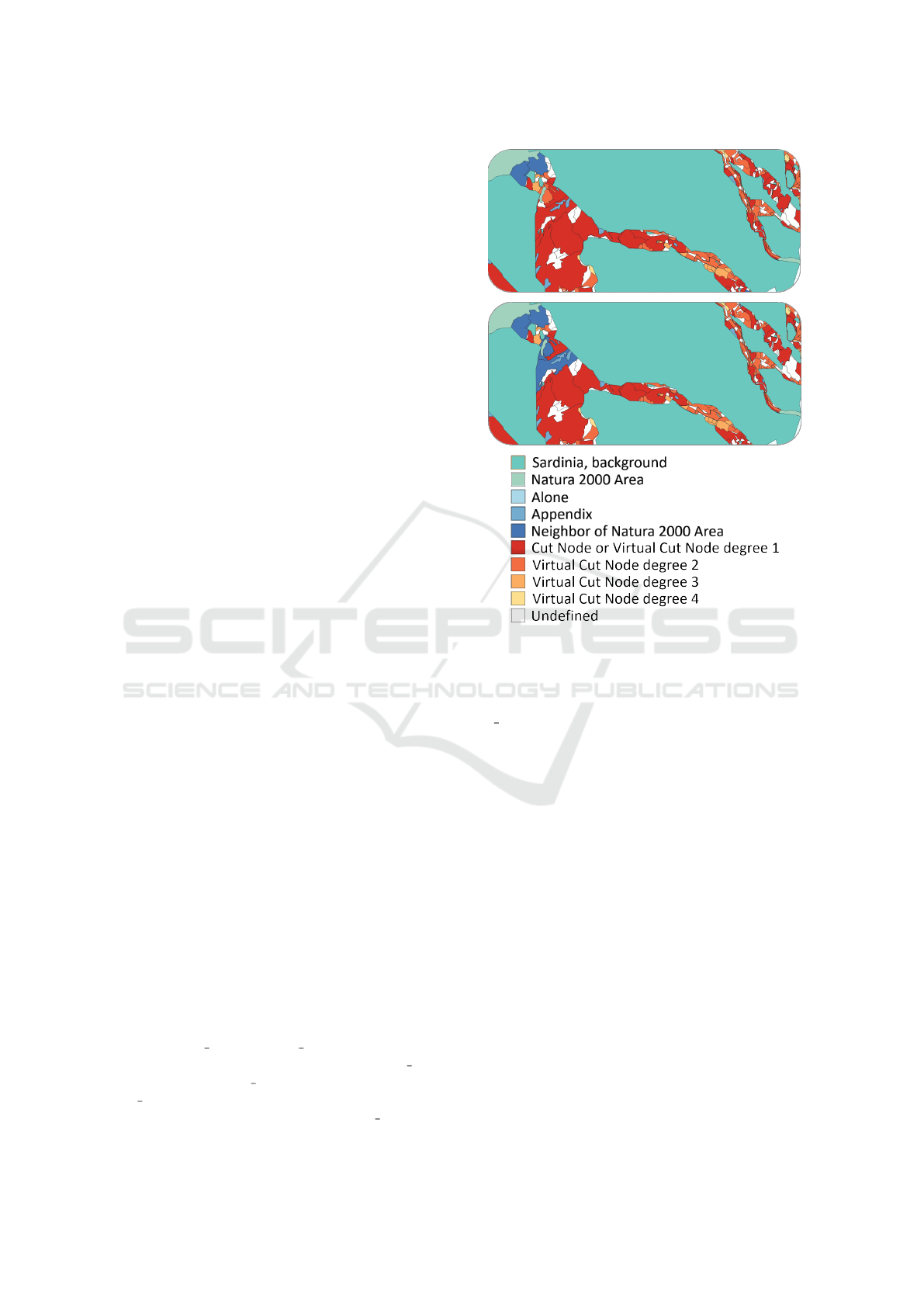
Figure 5: On top, a corridor calculated with an accuracy of

−5

and with a max distance of 3. At the Bottom, the same

corridor calculated with an accuracy of 10

−20

and with a

max distance of 10.

sp score will get a combined value that will give a

clearer idea of the most critical and simultaneously

most visited nodes, as visible in Figure 6.

3 CONCLUSION AND FUTURE

WORKS

The study of ecological networks is an increasingly

important topic to be analyzed. ECGraph has demon-

strated with its performances and results that it can be

an useful support tool in the study of the viability of

the ecological network, ﬁnding the different paths and

their critical patches.

Like many problems of complex networks, even

the one exposed is highly susceptible to the size and

conformation of the network given as input. As has

been explained, different parts of the algorithm have

a quadratic time complexity, which takes longer to

compute as the required precision increases. Despite

that, there is still room for improvement both in the

data structures used in the execution of the program

COMPLEXIS 2021 - 6th International Conference on Complexity, Future Information Systems and Risk

Table 1: The time needed to compute the algorithm with the different Accuracy and Max Distance settings. The vcn degree

ALONE, APPENDIX, and cut node all execute under one second.

Accuracy Max Distance Areas Shortest Path VCN d2 VCN d3 VCN d4

−5

3 45s 2m 50s 1m 20s 10m 59s 53m 12s

−20

10 1h 16m 46s 6m 24s 2m 48s 15m 49s 1h 7m 55s

Table 2: Type and number of nodes found.

Alone Appendix Neighbor Area Cut node VCN d3 VCN d3 VCN d4

38 873 373 475 1362 454 203

38 823 549 471 1350 445 206

Figure 6: The Figure expresses the score from 0 to 1. On

top, there is a corridor with no shortest path, as it does not

connect areas, and so entirely white. At the bottom, instead,

there is a corridor with several critical areas as they are fre-

quently used and simultaneously cut nodes.

and the implementation of the algorithms exposed.

In its most simpliﬁed version, with a relatively low

runtime on a commercial computer, ECGraph allows

establishing the network structure up to the virtual cut

nodes of second degree. The customization of the in-

put values and even more the open source nature of

the project allow having a solid starting point for the

development of even more useful tools.

As a demonstration of this, a software that can be

integrated with ECGraph is already in phase of devel-

opment, which will allow to have a graphic interface

designed for the representation of the data exposed,

and can even give more speciﬁc additional informa-

tion, such as the virtual cut nodes generated by the se-

lected parent node, the corridor change when a node

is removed and other useful data in real time.

Ultimately, the creation of a community that can

provide feedbacks and ecological corridors ﬁles for

the software improvement would allow reﬁning the

tool more and more, making it more powerful, robust,

and even easier to use.

ACKNOWLEDGEMENTS

This paper is written within the Research Program

”Paesaggi rurali della Sardegna: pianiﬁcazione di in-

frastrutture verdi e blu e di reti territoriali complesse

- CUP: J86C17000180002 - Progetto di ricerca di

base dell’Universit

a di Sassari e Cagliari ﬁnanziato

sul Fondo di Sviluppo e Coesione 2014-2020”. The

research leading to these results has received funding

from the Autonomous Region of Sardinia (Legge Re-

gionale 7/2007).

REFERENCES

Bodini, A. and Cossu, Q. (2010). Vulnerability assess-

ment of central-east sardinia (italy) to extreme rainfall

events. Natural Hazards and Earth System Sciences,

10(1):61–72.

Butler, H., Daly, M., Doyle, A., Gillies, S., Hagen, S.,

Schaub, T., et al. (2016). The geojson format. Internet

Engineering Task Force (IETF).

Cannas, I. and Zoppi, C. (2017). Ecosystem services and

the natura 2000 network: a study concerning a green

infrastructure based on ecological corridors in the

metropolitan city of cagliari. In International Confer-

ence on Computational Science and Its Applications,

pages 379–400. Springer.

Dijkstra, E. W. et al. (1959). A note on two problems

in connexion with graphs. Numerische mathematik,

1(1):269–271.

Evans, D. (2012). Building the european union’s natura

2000 network. Nature conservation, 1:11.

Fenu, G. and Nitti, M. (2011). Strategies to carry and for-

ward packets in vanet. In International Conference on

Digital Information and Communication Technology

and Its Applications, pages 662–674. Springer.

Fenu, G. and Pau, P. L. (2015). Evaluating complex network

indices for vulnerability analysis of a territorial power

ECGraph: A Complex Networks Tool to Classify Critical Points of Ecological Corridors

grid. Journal of Ambient Intelligence and Humanized

Computing, 6(3):297–306.

Fenu, G. and Pau, P. L. (2018). Connectivity analysis of

ecological landscape networks by cut node ranking.

Applied network science, 3(1):22.

Fenu, G. and Podda, E. (2020). A model of second-

degree virtual cut nodes applied to complex networks

in ecological landscape. Procedia Computer Science,

170:123–128.

Gill Jr, R. E., Tibbitts, T. L., Douglas, D. C., Handel, C. M.,

Mulcahy, D. M., Gottschalck, J. C., Warnock, N., Mc-

Caffery, B. J., Battley, P. F., and Piersma, T. (2009).

Extreme endurance ﬂights by landbirds crossing the

paciﬁc ocean: ecological corridor rather than barrier?

Proceedings of the Royal Society B: Biological Sci-

ences, 276(1656):447–457.

Jenson, S. K. and Domingue, J. O. (1988). Extracting topo-

graphic structure from digital elevation data for ge-

ographic information system analysis. Photogram-

metric engineering and remote sensing, 54(11):1593–

1600.

Jongman, R. H. (1995). Nature conservation planning in

europe: developing ecological networks. Landscape

and urban planning, 32(3):169–183.

Orda, L. D., Jensen, T. V., Gehrke, O., and Bindner, H. W.

(2019). Efﬁcient routing for overlay networks in a

smart grid context. In SMARTGREENS, pages 131–

136.

Ostermann, O. P. (1998). The need for management of na-

ture conservation sites designated under natura 2000.

Journal of applied ecology, 35(6):968–973.

Severance, C. (2012). Discovering javascript object nota-

tion. Computer, 45(4):6–8.

Team, Q. D. et al. (2015). Qgis geographic information sys-

tem. open source geospatial foundation project. URL:

http://qgis. osgeo. org.

Tilkov, S. and Vinoski, S. (2010). Node. js: Using javascript

to build high-performance network programs. IEEE

Internet Computing, 14(6):80–83.

Urban, D. and Keitt, T. (2001). Landscape connectivity:

a graph-theoretic perspective. Ecology, 82(5):1205–

1218.

COMPLEXIS 2021 - 6th International Conference on Complexity, Future Information Systems and Risk