Comparison between Filtered Canny Edge Detector and

Convolutional Neural Network for Real Time Lane Detection in a

Unity 3D Simulator

Jurij Kuzmic and Günter Rudolph

Department of Computer Science, TU Dortmund University, Otto-Hahn-Str. 14, Dortmund, Germany

Keywords: Lane Detection, Convolutional Neural Network (ConvNet), Filtered Canny Edge Algorithm, Autonomous

Driving, Simulator in Unity 3D, Sim-to-Real Transfer, Training Data Generation, Computational Intelligence.

Abstract: This paper presents two methods for lane detection in a 2D image. Additionally, we implemented filtered

Canny edge detection and convolutional neural network (ConvNet) to compare these for lane detection in a

Unity 3D simulator. In the beginning, related work of this paper is discussed. Furthermore, we extended the

Canny edge detection algorithm with a filter especially designed for lane detection. Additionally, an optimal

configuration of the parameters for the convolutional neural network is found. The network structure of the

ConvNet is also shown and explained layer by layer. As well known, a lot of annotated training data for

supervised learning of ConvNet is necessary. These annotated training data are generated with the Unity 3D

environment. The procedure for generation of annotated training data is also presented in this paper.

Additionally, these two developed systems are compared to find a better and faster system for lane detection

in a simulator. Through the experiments described in this paper the comparison of the run time of the

algorithms and the run time depending on the image size is presented. Finally, further research and work in

this area are discussed.

1 INTRODUCTION

In the autonomous vehicle industry, vehicles can

drive independently and without a driver. To do this,

these vehicles have to recognise the lane precisely in

order not to get away from the road and not to injure

the occupants. The lane markings are marked as solid

or dashed lines on the left and right side of the road

and are directly visible to the human eye. But for

autonomous vehicles we need algorithms. These lines

of the lane have to be distinguished and separated

from other lines in the image by the autonomous

vehicle. After the separation of the lines in a 2D

image, the centre of the lane can be calculated next.

Lane detection is not new and has been researched in

the vehicle industry for a long time. Today, Lane

Keeping Assist Systems (LKAS) or Lane Departure

Warning Systems (LDWS) are standard equipment in

some vehicles. These systems warn if you get out of

lane or can even keep the car in the lane for a while.

For example, at Nissan Motors such systems exist

since 2001 (Tsuda, 2001), at Citroën since 2005

(Web.archive, 2005) and at Audi since 2007

(Audiworld, 2007). The problem in academic

research is that algorithms and procedures, which are

already established in the autonomous vehicle

industry, are kept under lock and key and are not

freely accessible. For this reason, own algorithms and

procedures have to be researched and developed in

the academic field.

The goal of our work is to switch from the

simulation we have developed before (Kuzmic and

Rudolph, 2020) to the real model cars. In case of a

successful transfer of simulation to reality (sim-to-

real transfer), the model car behaves exactly as before

in the simulation. In the simulation, some tools keep

the vehicle on track without visual evaluation. In

reality, these aids do not exist. For this reason, the

lane in the simulation also has to be recognised

visually with a camera. For this purpose, two methods

are implemented, tested and compared in this paper.

These methods can not only be applied to the images

from the simulation. After some adjustments of the

parameters, these methods are also suitable for real-

world use.

148

Kuzmic, J. and Rudolph, G.

Comparison between Filtered Canny Edge Detector and Convolutional Neural Network for Real Time Lane Detection in a Unity 3D Simulator.

DOI: 10.5220/0010383701480155

In Proceedings of the 6th Inter national Conference on Internet of Things, Big Data and Security (IoTBDS 2021), pages 148-155

ISBN: 978-989-758-504-3

2 RELATED WORK

There are some scientific papers dealing with the

detection of the lane, e.g. (Wang, Teoh, Shen, 2004)

who have made the detection of the lane and tracking

using B-Snake or (Kim, 2008) who has developed a

robust lane-detection-and-tracking algorithm to deal

with challenging scenarios such as a lane curvature or

worn lane markings. Some scientific works use the

Canny edge algorithm and hyperbola fitting to detect

the lane (Assidiq, Khalifa, Islam, Khan, 2008). A

fairly recent approach to detect lanes is to incorporate

information from previous frames. This can be

realised by combining the convolutional neural

network (CNN) and the recurrent neural network

(RNN) (Zou et al., 2020). As soon as 3D information

is available, it is possible to distinguish between roads

and obstacles (Nedevschi et al., 2004). Such 3D

information can be obtained, for example, from

LiDAR sensors (Beltrán et al., 2018). Another

approach to get 3D information for lane or object

detection is the stereo camera. This camera contains

two cameras at a certain distance, similar to human

eyes. This delivers two images. The two images can

be used to determine the depth of the image to

distinguish between roads, humans, cars, houses, etc.

(Li, Chen, Shen, 2019). Also, some related scientific

papers present the sim-to-real transfer. Most of them

are deep reinforcement learning approaches. The goal

of our work is to develop further methods for lane

detection in a simulator, to perform a sim-to-real

transfer and to switch from simulation to the real

model vehicles.

3 FILTERED CANNY EDGE FOR

LANE DETECTION

The Canny edge detector (Canny, 1986) is often used

to create edges in a 2D image because it works

quickly and accurately. In an image which shows a

track, the human eye directly detects the track. But to

keep a car in the lane, these lines have to be filtered

first. For this reason, we have extended this algorithm

and researched our procedure for filtering. To

determine the lane using the Canny edge detector, a

greyscale image has to be created from the coloured

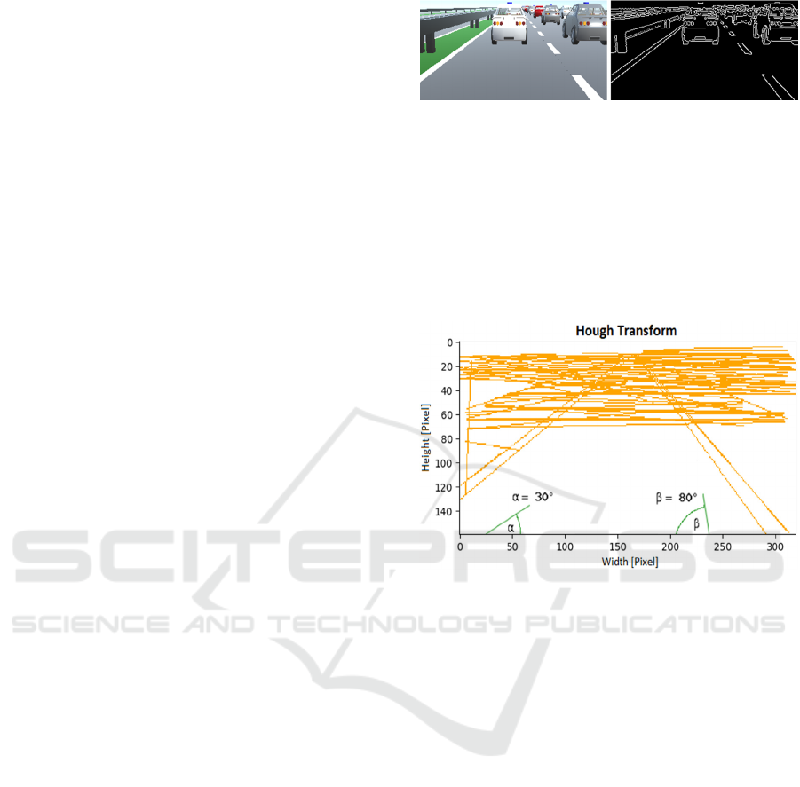
input image (Fig. 1, left). In the next step, an edge

image has to be made from the greyscale image using

the canny edge algorithm. Figure 1, right shows the

generated edge image from the coloured input image.

Figure 1: Image from the simulation. Left: Colour input

image. Right: Generated Canny edge image.

The edges can now be extracted as lines from the

created edge image using the Hough transform (Canu,

2018). This transformation gives the coordinates of

all lines in the image as P (x

, y

) and Q (x

, y

)

coordinates. Figure 2 shows all found lines from the

edge image with the Hough transform demonstrated

in a diagram.

Figure 2: Plotted coordinates of lines after Hough transform

(orange). Angles alpha and beta for comparison (green).

For each line, the gradient (m) of the straight line is

calculated. From this gradient, the angle in degrees to

the X-axis can now be calculated with the arctangent

function atan(m). After calculating the angles, all

lines with an angle below 30° and above 80° (alpha

and beta in Figure 2) can be ignored. These

parameters work for our orientation and tilt of the

camera in the simulation. If the position of the camera

changes, these parameters can be adjusted in this

algorithm. For all remaining (pre-filtered) lines the

intersections with the X-axis (IX) can now be

calculated and saved together with the P and Q

coordinates of the straight line. In the next step, the

smallest distance (D) on the X-axis has to be found

from the centre of the image (B) to the left and right:

D = |IX-B|. Search in a predefined radius (R) for

further intersection points (IX) to calculate the centre

of the lane marking. This parameter depends on the

width of the image (pixels) and can also be adjusted.

The following figure 3 shows this procedure.

Comparison between Filtered Canny Edge Detector and Convolutional Neural Network for Real Time Lane Detection in a Unity 3D

Simulator

149

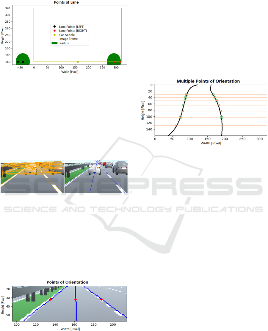
Figure 3: Filtered lane points (IX). Found lane points left

(black) and right (red) in a certain radius (dark-green). The

input image frame and the middle of the vehicle (light-

green).

So, an average function left and right can be

calculated from the found lines. These intermediate

functions are the course of the track marking left and

right. To calculate the centre of the track, the centre

can be calculated from these two average functions.

The following figure 4 shows the lane before (Fig. 4,

left) and after filtering (Fig. 4, right).

Figure 4: Filtered Canny edge for lane detection. Left:

Plotted lines after Hough transform in a colour input image.

Right: Colour input image with filtered lane detection.

In this example, it was assumed that the track is

straight. On motorways, this is usually the case. At

least in the relevant vicinity of the car. Actually, the

motorways are only slightly curved. If the road is

straight, only one orientation point left and right at a

certain height (red points in figure 5) is sufficient to

determine the lane course in the input image and to

control the vehicle.

Figure 5: Points of orientation at a certain height (red

points) to calculate the centre of the lane and to keep the

vehicle on track (controlling the car).

However, if the road is curved, several orientation

points at different heights are necessary. For this

purpose, the image can be divided horizontally into

several sections (Wang, Teoh, Shen, 2004). The

number and height of the sections can be freely

chosen. This horizontal split depends on the

resolution, the visible image area and the tilt of the

camera. As soon as the splitting is done, the lane

markings left and right of each section can be

recognised as a straight line with the filtered Canny

edge algorithm. The following Figure 6 describes this

procedure. The individual sections are separated by

the horizontal orange lines.

Figure 6: Multiple points of orientation for controlling the

car. Section separator (orange lines). Points of orientation

(green squares).

After the lane detection for each section, the track

markings are obtained as 2D coordinates left and right

of the image. Thus, the lane centre can be determined

or the course of the track can be approximated as a

function.

Our filtered Canny edge algorithm at a glance:

0. As a preliminary work, the camera should be

aligned and calibrated. Only the vital areas

should be visible in the image (only the

track). For example, the bonnet of the car or

the power lines in the sky should not be

visible.

1. Create a greyscale image from the coloured

input image.

2. Create a Canny edge image from the

grayscale image.

3. Apply Hough transform to the edge image

(2D coordinates for P and Q).

4. Calculate the gradient (m) for each straight

line.

5. Calculate the angle with atan(m) from the

gradient (m).

6. Ignore all lines with an angle below 30° and

above 80°.

7. Calculate the points of intersection with the

X-axis (IX) for the remaining lines.

8. Save intersection points (IX) with the P and

Q 2D coordinates.

IoTBDS 2021 - 6th International Conference on Internet of Things, Big Data and Security

150

9. From the centre of the image (B), find the

smallest distance D = |IX-B| left and right.

10. Search in a predefined radius (R) for further

intersection points (IX) left and right.

11. Calculate an average function (straight line)

left and right from the found lines.

12. Calculate the centre of the track from these

two functions left and right.

4 ConvNet FOR LANE

DETECTION

To train a convolutional neural network (ConvNet)

optimally, a large number of annotated data points

(training data) are required for supervised learning.

Such data can also be created manually. However,

with so many data points, annotation takes a very long

time. Depending on the application, different data are

also required. The amount of training data, the input

and output data are also different. The CULane

dataset (Pan, Shi, Luo, Wang, Tang, 2018) offers data

for lane recognition for academic research. These

have already been manually annotated. However, for

further research, to perform a sim-to-real transfer, the

simulation has to be adapted to the real application.

In our case, the camera in the simulation has to have

the same resolution and orientation as the camera in

the model vehicle. For this reason, we have created

our own automatically annotated data set. The next

chapter describes this procedure.

4.1 Data Set

With our simulator in Unity 3D (Kuzmic and

Rudolph, 2020), thousands of annotated training data

(input and output data) could be generated

automatically. For the automatic generation of the

required data sets, two cameras were installed in the

vehicle at the same place in the simulator. The first

camera could see the environment normally (Fig. 7,

left), the second camera could only see the lane

markings left and right (Fig. 7, right).

Figure 7: Camera images of the vehicle. Left: Camera for

input images. Right: Camera for output images (only lane

markings).

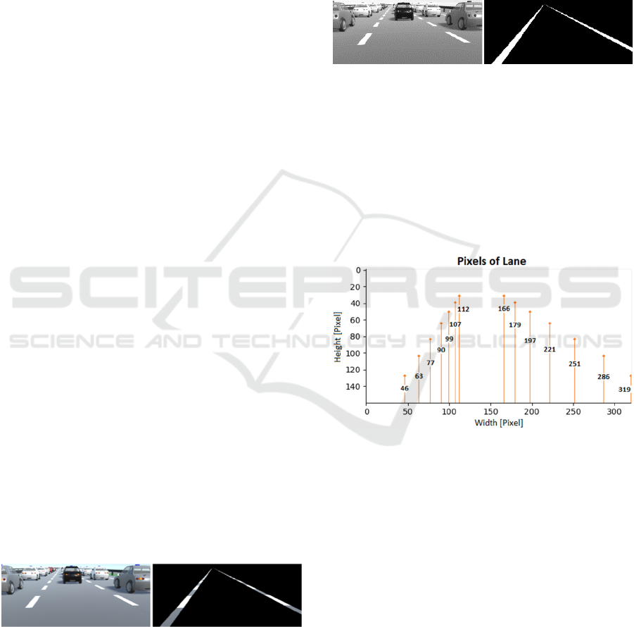
These two images (Fig. 7) could be used for the

further generation of the training data. The input

image (Fig. 8, left) for the ConvNet was created from

Figure 7, left. This was additionally converted into a

greyscale image. To get the annotated data (output

data), a binary image (Fig. 8, right) was created first

from figure 7, right. For this purpose, a threshold had

to be found and adjusted for the simulated images

(Al-amri, Kalyankar, Khamitkar, 2010). This

parameter depends on the strength of the different

light influences in the image.

Figure 8: Input and binary image for training. Left:

Grayscale input image. Right: Binary image for annotation.

From this binary image, the information for the left

and right lane marking could be extracted (Fig. 9).

The first step is to find the centre of the lane markings

at a certain height. Since the heights are predefined

(Y-coordinates), only the X-coordinate of these pixels

is used as annotation for the input image (Fig. 8, left).

In this case, the neural network has 14 outputs; one

for each class.

Figure 9: Coordinates of the track sequence for annotation

of the input image.

As explained in section 3, several orientation points

should be defined for a winding road. For this reason,

we have defined seven different heights to describe

the straight or curved lane. These heights (32, 40, 52,

66, 84, 104, 128) are important for the orientation of

the camera and in our case, they are always the same

for our camera. The following X-coordinates (46,

319, 63, 286, 77, 251, 90, 221, 99, 197, 107, 179, 112,

166) could be extracted from figure 9 from bottom to

top. These X-positions serve as annotation for the

input image (Fig. 8, left). Due to the fast generation

of the training data, images with different width and

height can be generated and automatically annotated.

The following data sets were created and tested

(width x height): 160x80, 320x160, 640x160 and

Comparison between Filtered Canny Edge Detector and Convolutional Neural Network for Real Time Lane Detection in a Unity 3D

Simulator

151

640x320 pixels. A total of about 100,000 data sets

were created. Due to the automatic generation of the

images, the data set contains colour images (RGB

images), greyscale images and binary images as input

with the corresponding annotation.

4.2 Network Architecture

After a long period of training, evaluation and testing,

we found an optimal configuration for the ConvNet

for our training data. The convolutional layers are

characterized by the parameters output, kernel and

stride. Output is the number of output filters in the

convolution. Kernel is specifying the height and

width of the 2D convolution window which moves

over the pixels in the input image. Stride is specifying

the steps of the convolution along with the height and

width and is almost always symmetrical in the

dimension (TensorFlow, 2020). We used Rectified

Linear Unit (ReLU) as an activation function for all

layers. In the last dense layer (fully connected layer),

we used a linear function as activation for regression.

The convolutional neural network is structured as

follows (Winkel, 2020):

 Convolutional (8, k = (5, 5), s = (2, 2))

 2 x Convolutional (8, k = (3, 3), s = (1, 1))

 Dropout (0.5)

 Convolutional (16, k = (5, 5), s = (2, 2))

 2 x Convolutional (16, k = (3, 3), s = (1, 1))

 Dropout (0.5)

 Convolutional (32, k = (5, 5), s = (2, 2))

 2 x Convolutional (32, k = (3, 3), s = (1, 1))

 Dropout (0.5)

 Convolutional (64, k = (5, 5), s = (2, 2))

 2 x Convolutional (64, k = (3, 3), s = (1, 1))

 Dropout (0.5)

 Flatten

 Dense (2000)

 Dense (1000)

 Dense (200)

 Dense (14)

The last dense layer shows the number of outputs of

the neural network. In our example, this contains 14

outputs for each X-coordinate of the lane (see section

4.1). The experiments with the convolutional neural

network are discussed next.

5 EXPERIMENTS

The following experiments were carried out to

compare the functionality and the run time of filtered

Canny edge algorithm and ConvNet for lane

detection. The resolution is in the format width x

height. All experiments (training of the ConvNet and

the run time measurements) are carried out on the

same hardware: Intel i7-9750H, 16 GB DDR4, 256

GB SSD, NVIDIA GeForce GTX 1660 Ti. This gives

the possibility to compare the results afterwards. The

input images for the respective methods are also the

same.

5.1 Filtered Canny Edge for Lane

Detection

The following Table 1 shows the run time of the

filtered Canny edge algorithm compared to the size of

the input image. The size of the section in the image

was evenly split. For an image with 160x80 pixels, it

corresponds to a section size of 10 pixels in height.

The time measurement per image is given in

milliseconds. Since the determination of the lines in

an image per section is different. So the average time

for the calculation of the section was built. Through

the input image is split into sections once, the time for

splitting (ct) is calculated only once. The run time (t)

in table 1 results from 𝑡=𝑠𝑡•𝑠+𝑐𝑡.

Table 1: Run time of the filtered Canny edge detection

algorithm for lane detection. First column contains the

number of the experiment (Exp. No.).

Exp.

No.

Resolution

[Pixel]

Section

(s)

Crop

[ms] (ct)

Section

Time

[ms] (st)

Run

Time

[ms] (t)

1 160x80

0 2.99 2.99

2 320x160 0 6.00 6.00

3 640x160 0 9.97 9.97

4 640x320 0 12.98 12.98

5 160x80

< 0.01 0.37 2.97

6 320x160 < 0.01 0.74 5.93

7 640x160 0.96 1.99 16.88

8 640x320 1.00 2.62 21.96

The various experiments have shown that larger

images provide more accurate lane detection. But,

finding the lane in this input image also takes longer.

If the resolution is doubling, the run time for finding

the lane in this image is doubling, too (comparison of

the run times no. 1 and 2 in table 1). For this reason,

we have chosen the resolution 320x160 pixels as the

optimal resolution for lane detection for our data. In

straight and curved roads, the evaluation takes about

six milliseconds per frame from the input image

(comparison of the run times no. 2 and 6 in table 1).

5.2 ConvNet for Lane Detection

The first step is to find the optimal input for the

convolutional neural network. Colour images,

greyscale images and binary images are available for

this purpose. To decide for one of these images, the

IoTBDS 2021 - 6th International Conference on Internet of Things, Big Data and Security

152

neural network has to be trained with these images

and the results have to be compared afterwards. By

mixing (shuffle) the data sets, each run of training is

different. The best model from ten training runs is

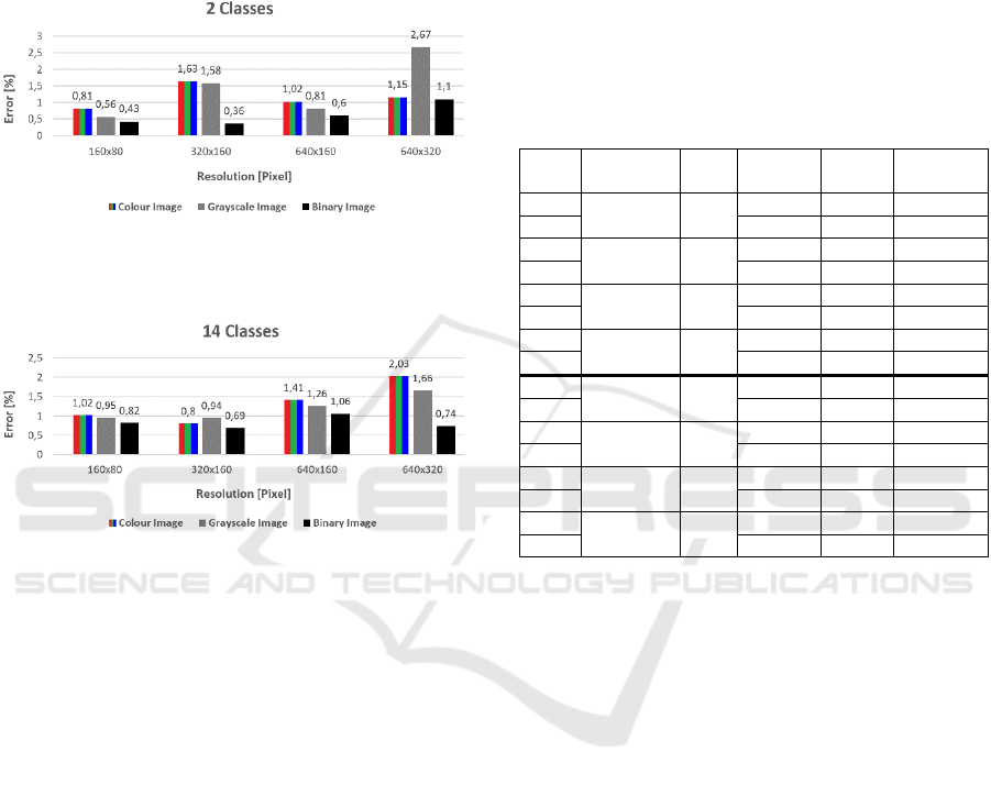
evaluated. The error is given in per cent and per class.

To compare the errors on different image sizes, this

error is calculated with the image width (pixels).

Figure 10: Diagram of training the ConvNet with two

classes. Error in per cent after ten training times with

different image resolution. The smallest value is the best.

Figure 11: Diagram of training the ConvNet with 14

classes. Error in per cent after ten training times with

different image resolution. The smallest value is the best.

As can be seen on these two diagrams, the models

trained with the binary images provide better

(smaller) error rates. This is the case for 2 (Fig. 10)

and 14 classes (Fig. 11). However, these models can

only be used in the simulation. Because of the

different light influences in the real image, the

threshold for the creation of the binary images has to

be found and adjusted every frame. This is not the

case with the simulated images. Also, the various

experiments have shown that models with the

greyscale image as input usually result in a higher

regression accuracy than the input with RGB images.

Depending on the use case, this result can be

confirmed (Bui et al., 2016). This result also depends

on the nature of images to be classified (Yadav,

2015). As soon as more information is needed from

the images, a colour image can sometimes achieve

better results than a greyscale image. Let us now look

at the colour and greyscale image models. It can be

seen that the model trained with greyscale images

with two classes as output and the 160x80 pixels

resolution provides the smallest error. So it is more

accurate compared to other models with two classes.

With 14 classes, the best result is achieved with the

model trained with colour images and the pixel size

320x160. After these experiments, the run time (Tab.

2) for the detection of the lane can be measured. For

this purpose, the best models of colour images and

greyscale images for the respective resolution are

tested. Classes 2 and 14 in table 2 correspond exactly

to sections 1 and 8 in table 1 of the experiments for

the filtered Canny edge for lane detection.

Table 2: Run time of the ConvNet for lane detection. First

column contains the number of the experiment (Exp. No.).

Exp.

No.

Resolution

[Pixel]

Class Model Error

[%]

Run Time

[ms]

160x80 2

Grey 0.56 18.15

2 Colour 0.81 17.95

320x160 2

Grey 1.58 18.95

4 Colour 1.63 19.05

640x160 2

Grey 0.81 19.65

6 Colour 1.02 20.75

640x320 2

Grey 2.67 22.64

8 Colour 1.15 27.33

160x80 14

Grey 0.95 18.45

10 Colour 1.02 17.80

320x160 14

Grey 0.94 18.85

12 Colour 0.80 20.05

640x160 14

Grey 1.26 19.65

14 Colour 1.41 21.09

640x320 14

Grey 1.66 22.25

16 Colour 2.03 25.04

In these experiments can be seen, that the number of

classes does not affect the run time (comparison of

run times no. 1 and 9 in table 2). The models with the

colour images as input require more run time

compared to the greyscale images as input to achieve

the desired output (comparison of the run times no.

15 and 16 in table 2). Because the greyscale images

have only one colour channel. In comparison, the

colour images have three colour channels. The run

time also increases for larger images compared to

smaller images as input (comparison of run times no.

1 and 15 in table 2). Since the kernel of the

convolutional layer passes through more pixels in the

input image. Also, the error of the trained model does

not affect the run time (comparison of the run times

no. 7 and 8 in table 2).

5.3 Evaluation of Results

After the performance tests for the filtered Canny

edge detection and the convolutional neural network,

these two procedures can be compared and evaluated.

The filtered Canny edge algorithm needs approx. 6

milliseconds (ms) to detect the lane in a 320x160

Comparison between Filtered Canny Edge Detector and Convolutional Neural Network for Real Time Lane Detection in a Unity 3D

Simulator

153

pixel image. With a video recording of 30 frames per

second (FPS), the actual frame rate decreases because

6 additional milliseconds are needed to determine the

lane per frame (6 𝑚𝑠 • 30 = 180 𝑚𝑠). The System

needs approx. 1.18 seconds to process 30 frames.

Calculated to the frames per second, it is around 25

FPS. The ConvNet needs about 19 ms to determine

the lane in a 320x160 pixel greyscale image with our

computer hardware. Additionally, this procedure

requires 570 ms per 30 frames (19 𝑚𝑠 • 30 =

570 𝑚𝑠). This reduces the actual frame rate to about

19 FPS. Some front cameras installed in self-driving

cars in the automotive industry can record 1080p

videos at up to 60 FPS (Texas Instruments, 2021).

This means, up to 44 FPS for filtered Canny edge

method and 28 FPS for ConvNet could be achieved.

The following calculations depend on the hardware of

the system. As a standard, videos with a lot of motion

are recorded at 30 FPS (Brunner, 2017). Therefore,

both tested procedures are suitable for lane detection.

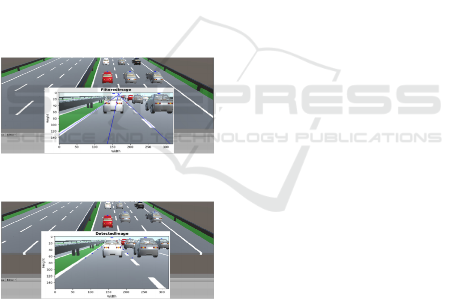
Both models (Fig. 12 and Fig. 13) are successfully

tested in the simulator. The plot of the lane is taken

from the camera of the red vehicle.

Figure 12: Testing of filtered Canny edge for lane detection

in the simulator. The plot of the lane is taken from the

camera of the red vehicle.

Figure 13: Testing of ConvNet for lane detection in the

simulator. The plot of the lane is taken from the camera of

the red vehicle.

The evaluation of the results gives the following

advantages for the filtered Canny edge method

compared to the ConvNet: Faster detection of the lane

(factor of 3 on our hardware), no training of the

artificial neural network, no training data necessary,

after adjusting the parameters - ready for different

camera orientations.

6 CONCLUSIONS

This section summarizes once again the points that

were introduced in this paper. Two methods are

presented and tested for the detection of the lane. The

first method is the Canny edge detector, which has

been extended by us. This is called filtered Canny

edge for lane detection. The lines are extracted from

an edge image and filtered under certain parameters.

This method can be used for straight and curved

roads. For curved roads, the input image can be split

horizontally into several sections. This algorithm can

be applied to each of these sections to find the track.

The smaller sections give a more accurate

approximation of the lane course. The second method

is a convolutional neural network, which is trained to

recognise the course of the track. Seven heights

(vertical) are defined in a 2D image. At these heights,

the X-coordinates for the track left and right are taken

and given to the convolutional neural network for

training. So the output of the ConvNet is 14 output

values, which describe the lane on seven different

heights. The found network structure is also presented

to implement this method of lane detection. The

acquisition of automated annotated training data from

the simulation is also presented. Experiments are

carried out for both procedures to make comparisons

and to find a suitable system for lane detection for a

model vehicle. Both presented methods are suitable

for the detection of the lane in a 2D image in terms of

quality and performance. For example, at 30 FPS,

there would be no jerking in the detection of the track

for each individual frame.

7 FUTURE WORK

As already announced, the goal of our future work is

to carry out a sim-to-real transfer successfully. This

means that the simulated environment is completely

applied to a real model vehicle. Thus, the behaviour

of the vehicles in the simulation can be compared

with the behaviour of the model vehicles in reality.

Especially, it is exciting to see how much FPS the

model car can work with. An important aspect on

motorways is the automatic creation of an emergency

corridor for the rescue vehicles in the case of an

accident. It is exciting to see whether the model

vehicles can form an emergency corridor for the

IoTBDS 2021 - 6th International Conference on Internet of Things, Big Data and Security

154

rescue vehicles. For example, how do the model

vehicles behave if an accident occurs? What is the

behaviour of the car if the radar sensor unexpectedly

fails or there are unexpected obstacles on the road, for

example, a deer crossing? These questions can be

answered after the sim-to-real transfer.

REFERENCES

Al-amri, S. S., Kalyankar, N. V., Khamitkar, S. D., 2010.

Image Segmentation by Using Threshold Techniques.

Journal of Computing, Volume 2, Issue 5.

Assidiq, A. A., Khalifa, O. O., Islam, M. R., Khan, S., 2008.

Real time lane detection for autonomous vehicles.

Computer and Communication Engineering, ICCCE

2008, International Conference on Kuala Lumpur, pp.

82-88.

Audiworld, 2007. The Audi Q7 4.2 TDI. Audiworld.com.

[online]. Available at: https://www.audiworld.com/

articles/the-audi-q7-4-2-tdi/. Accessed: 22/10/2020.

Beltrán, J., Guindel, C., Moreno, F. M., Cruzado, D.,

García, F., De La Escalera, A., 2018. BirdNet: A 3D

Object Detection Framework from LiDAR Information.

2018 21st International Conference on Intelligent

Transportation Systems (ITSC), IEEE, ISBN 978-1-

7281-0324-2.

Brunner, D., 2017. Frame Rate: A Beginner’s Guide.

Techsmith.com. [online]. Available at:

https://www.techsmith.com/blog/frame-rate-

beginners-guide/#:~:text=they're%20used.-

,24fps,and%20viewed%20at%2024%20fps. Accessed:

21/11/2020.

Bui, H. M., Lech, M., Cheng, E., Nelille, K., Burnett, I. S,

2016. Using grayscale images for object recognition

with convolutional-recursive neural network. In

Proceedings of the IEEE 6th International Conference

on Communications and Electronics, pp. 321-325.

Canny, J., 1986. A Computational Approach to Edge

Detection. IEEE Transactions on Pattern Analysis and

Machine Intelligence, Volume PAMI-8, No 6, pp. 679-

698.

Canu, S., 2018. Lines detection with Hough Transform –

OpenCV 3.4 with python 3 Tutorial 21. Pysource.com.

[online]. Available at: https://pysource.com

/2018/03/07/lines-detection-with-hough-transform-

opencv-3-4-with-python-3-tutorial-21/. Accessed:

15/09/2020.

Kahn, G., Abbeel, P., Levine, S., 2020. LaND: Learning to

Navigate from Disengagements. arXiv: 2010.04689

Kim, Z. W., 2008. Robust Lane Detection and Tracking in

Challenging Scenarios. IEEE Trans IEEE Transactions

on Intelligent Transportation Systems, Volume 9, Issue

1, pp. 16-26.

Kuzmic, J., Rudolph, G., 2020. Unity 3D Simulator of

Autonomous Motorway Traffic Applied to Emergency

Corridor Building. In Proceedings of the 5th

International Conference on Internet of Things, Big

Data and Security (IoTBDS), Volume 1: IoTBDS,

ISBN 978-989-758-426-8, pp. 197-204.

Li, P., Chen, X., Shen, S., 2019. Stereo R-CNN Based 3D

Object Detection for Autonomous Driving. Proceedings

of the IEEE/CVF Conference on Computer Vision and

Pattern Recognition (CVPR), pp. 7644-7652.

Nedevschi, S., Schmidt, R., Graf, T., Danescu, R., Frentui,

D., Marita, T., Oniga, F., Pocol, C., 2004. 3D lane

detection system based on stereovision. Intelligent

Transportation Systems. In Proceedings of the 7th

International IEEE Conference, pp. 161-166.

Pan, X., Shi, J., Luo, P., Wang, X., Tang, X., 2018. Spatial

As Deep: Spatial CNN for Traffic Scene

Understanding. AAAI Conference on Artificial

Intelligence (AAAI).

Tan, J., Zhang, T., Coumans, E., Iscen, A., Bai, Y., Hafner,

D., Bohez, S., Vanhoucke V., 2018. Sim-To-Real:

Learning Agile Locomotion For Quadruped Robots.

Proceedings of Robotics: Science and System XIV,

ISBN 978-0-9923747-4-7.

TensorFlow, 2020. TensorFlow Core v2.3.0 -

tf.keras.layers.Conv2D. Tensorflow.org. [online].

Available at: https://www.tensorflow.org/api_docs/

python/tf/keras/layers/Conv2D. Accessed: 13/09/2020.

Texas Instruments, 2021. Front camera. Automotive front

camera integrated circuits and reference designs.

Camera SerDes (DS90UB953-Q1). Ti.com. [online].

Available at: https://www.ti.com/solution/automotive-

front-camera. Accessed: 09/02/2021.

Tsuda, H., 2001. Nissan Demos New Lane Keeping

Products. Web.archive.org. [online]. Available at:

https://web.archive.org/web/20050110073214/http://iv

source.net/archivep/2001/feb/010212_nissandemo.htm

l. Accessed: 22/10/2020.

Wang, Y., Teoh, E. K., Shen, D., 2004. Lane detection and

tracking using B-Snake. Image and Vision Computing,

Volume 22, Issue 4, pp. 269-280.

Web.archive, 2005. Avoiding accidents. Webarchive.org.

[online]. Available at: https://web.archive.org/web

/20051017024140/http://www.developpement-

durable.psa.fr/en/realisation.php?niv1=5&niv2=52&ni

v3=2&id=2708. Accessed: 22/10/2020.

Winkel, S., 2020. Efficient lane detection for model cars in

simulation and in reality (German: Effiziente

Spurerkennung für Modellautos in Simulation und

Realität). Bachelor’s thesis, TU Dortmund University.

Yadav, P., 2015. Re: Which is best for image classification,

RGB or grayscale?. Researchgate.net. [online].

Available at: https://www.researchgate.net/post/

Which_is_best_for_image_classification_RGB_or_gra

yscale/55e962155dbbbd562d8b4591/citation/downloa

d. Accessed: 24/11/2020.

Zou, Q., Jiang, H., Dai, Q., Yue, Y., Chen, L., Wang, Q.,

2020. Robust Lane Detection from Continuous Driving

Scenes Using Deep Neural Networks. IEEE

Transactions on Vehicular Technology, Volume 69,

Issue 1, pp. 41-54.

Comparison between Filtered Canny Edge Detector and Convolutional Neural Network for Real Time Lane Detection in a Unity 3D

Simulator

155