Using Machine Learning to Forecast Air and Water Quality

Carolina Silva

, Bruno Fernandes

, Pedro Oliveira

and Paulo Novais

Department of Informatics, ALGORITMI Centre, University of Minho, Braga, Portugal

Keywords:

Environmental Sustainability, Machine Learning, Tree-based Models, Deep Learning.

Abstract:

Environmental sustainability is one of the biggest concerns nowadays. With increasingly latent negative im-

pacts, it is substantiated that future generations may be compromised. The research here presented addresses

this topic, focusing on air quality and atmospheric pollution, in particular the Ultraviolet index and Carbon

Monoxide air concentration, as well as water issues regarding Wastewater Treatment Plants, in particular the

pH of water. A set of Machine Learning regressors and classiﬁers are conceived, tuned, and evaluated in regard

to their ability to forecast several parameters of interest. The experimented models include Decision Trees,

Random Forests, Multilayer Perceptrons, and Long Short-Term Memory networks. The obtained results as-

sert the strong ability of LSTMs to forecast air pollutants, with all models presenting similar results when the

subject was the pH of water.

1 INTRODUCTION

Over the last few years, more data have been gener-

ated than ever. Consequently, many organizations,

whether business or public entities, identiﬁes data

as a valuable asset that supports its decision-making

process ((Hino et al., 2018; Sandryhaila and Moura,

2014)). On the other hand, Machine Learning (ML), a

ﬁeld from Artiﬁcial Intelligence (AI), has been grow-

ing in importance in the last decade ((Qiu et al.,

2016)). This ﬁeld concerns data collection, analysis,

and then the prediction of several meaningful param-

eters. ML is used in many sectors nowadays, once it

is recognized as a ﬁeld that can provide accurate and

real-time solutions. The various entities that operate

in the most diverse areas can, with ML, acquire the

ability to act before something occur, avoiding and

preventing negative impacts ((Qiu et al., 2016)).

Since ML can be implemented in a vast range

of areas, it is interesting to apply it in a way that

can make a difference, aiming for the common good.

From this emerges an area with important societal im-

pact: environmental sustainability. Sustainable de-

velopment, from an environmental point of view, has

been a signiﬁcant problem for countries for decades

since negative environmental impacts are increasingly

https://orcid.org/0000-0001-8585-5195

https://orcid.org/0000-0003-1561-2897

https://orcid.org/0000-0001-7143-5413

https://orcid.org/0000-0002-3549-0754

perceived and veriﬁed ((Isabel Molina-G

omez et al.,

2020)). Due to the registered population growth,

the demand for natural resources has, consequently,

raised. Further, industrial activities are increasingly

pronounced in developed countries, being the key to

their economic sustainability. All of this generates

anthropogenic emissions, which damage the environ-

ment, causing visible impacts such as public health

problems, climatic changes, and many others. All this

can compromise future generations. To avoid these

risks, responsible entities need to make decisions to

reduce its negative impacts and consequent hazard for

the population ((Sarkodie, 2021)).

Aiming to address important points on the scope

of environmental sustainability, this research focuses

on the conception, tuning, and evaluation of multiple

ML models to anticipate possible problematic situa-

tions. Thus, it allows one to act in a preventive way

to provide the best for the population and future gen-

erations. Further, it allows one to better allocate re-

sources and consequently, maximize potential bene-

ﬁts for companies as well as the human being.

Throughout this research, the CRISP-DM

methodology was the one being followed to ensure

a proper progress of this study. Overall, the main

goals of this research are to: (1) Forecast parameters

in the air quality domain, including the Ultraviolet

(UV) index and the Carbon Monoxide (CO) air

concentration; (2) Forecast parameters in the water

quality domain, in particular the pH of water, con-

1210

Silva, C., Fernandes, B., Oliveira, P. and Novais, P.

Using Machine Learning to Forecast Air and Water Quality.

DOI: 10.5220/0010379312101217

In Proceedings of the 13th International Conference on Agents and Artiﬁcial Intelligence (ICAART 2021) - Volume 2, pages 1210-1217

ISBN: 978-989-758-484-8

cerning Wastewater Treatment Plants (WWTPs),

in the exact moment before it returns to natural

sources; (3) Perceive which are the relevant features

concerning the forecasting process, evaluated by the

quality of the outcomes generated by each model;

(4) Understand, compare, and tune tree-based models

(Decision Trees (DTs) and Random Forests (RFs)),

Multilayer Perceptrons (MLPs), and Long Short

Term-Memory networks (LSTMs).

The remaining of this paper is structured as fol-

lows: the next section describes the current state of

the art regarding the UV index and CO impacts, as

well as the WWTP context, exploring its operations

and the measured parameters. Material and meth-

ods are detailed in the following section, showing the

data exploration process, its preparation, and the used

technologies. The fourth section focuses on the con-

ducted experiments, showing the conceived scenarios

and the hyperparameters’ searching space. The ﬁfth

section discusses the obtained results. Finally, con-

clusions are drawn and future work is outlined.

2 STATE OF THE ART

Environmentally sustainability is a problem that cov-

ers the effort to establish green management, taking

into account current and future generations. Atmo-

spheric pollution, more speciﬁcally air pollution, is

an important environmental issue, primarily linked to

urban conditions and industrial emissions. This prob-

lem has grown, resulting from an increase in polluting

industries, making human activity its central source

((Cohen et al., 2017)). One of the most well recog-

nized primary pollutants is CO. This pollutant con-

stitutes a problem, causing some negative health im-

pacts. The biggest issue of CO exposure is tissue hy-

poxia (oxygen deﬁciency in tissues) due to its capa-

bility to bind the hemoglobin, blocking the tissues to

enough oxygen ((Lee et al., 2020)). Further, there

are other problems appointed for CO exposure such

as neurological sequels in humans, particularly neuro-

cognitive impairment and behavioral abnormalities in

children ((Block et al., 2012)).

UV radiation is yet another topic on air quality

that concerns the human health. Over the years, the

ozone layer has become thinner, leading to danger-

ous UV radiation reaching Earth’s surface. To in-

form the population of this radiation risk and cul-

tivate changes in mindset and attitudes against ex-

posure to the sun, the UV index was created ((Igoe

et al., 2013)). On a controlled scale, the UV radia-

tion has numerous beneﬁts: it suppresses stress, im-

proves sleep, prevents some illness, and increases the

production of vitamin D in the human body ((Nor-

val et al., 2011)). However, it may cause severe

health problems such as ocular melanoma, skin can-

cer (melanoma and non-melanoma skin cancers), and

premature skin aging when exposed to high UV levels

((Norval et al., 2011)).

Water is an indispensable resource for the human

being. It is used in many contexts: at home, indus-

tries, for agriculture, among many others. So, it is

crucial to understand what happens to the residual

water that results from that use. In fact, ﬁrst, wa-

ter is collected and transported to a plant in water

pipes (a network that connects the water sources to

the plant). Here, the residual water, commonly called

wastewater, is treated and returned to water sources in

environmentally safe conditions. This plant is called

a WWTP.

A WWTP has a crucial role in Environmental Sus-

tainability. There are four fundamental phases in

WWTPs operations. The ﬁrst one is known as the pre-

treatment, being here where coarse solids and ﬂoating

materials are removed from the wastewater. The sec-

ond is the primary treatment. At this phase, the re-

maining solids are removed as well as organic matter,

mainly by the action of gravity, using a primary clar-

iﬁer. Then, it occurs the secondary treatment, where

the biodegradable organic matter is removed, along

with suspended solids and nutrients. This phase can

be divided in two stages: (1) the aeration tank (the

anoxic and aerated zone) and (2) the secondary clar-

iﬁer. The last crucial phase is the tertiary treatment,

in which the remaining solids are removed, together

with organic matter and toxic compounds. After that,

the water is ready to be discharged to the surface. Ad-

ditionally, there is a sludge line in which the solids

that left from the previous steps are treated ((Spell-

man, 2013)). Figure 1 shows a simpliﬁed WWTP op-

eration process.

Within a WWTP, there are several parameters that

need to be controlled and evaluated in the different

stages of the operation process. Among these param-

eters one may ﬁnd the temperature, conductivity, al-

kalinity, pH, Nitrogen, dissolved oxygen, solids, bac-

teria, among others. However, one of the most signif-

icant wastewater characteristics is its pH. When less

than 5, it indicates acid water, while values higher

than 9 indicate it is alkaline. Identify the pH value in

a WWTP is essential since this is a controlling agent

of the biological and physical-chemical wastewater

functions. This parameter deserves special attention,

mainly in the aeration tank. Here occurs a biological

treatment, with the action of several microorganisms

that need the right pH conditions to do its job ((Spell-

man, 2013)). At the exit of a WWTP (the discharge

Using Machine Learning to Forecast Air and Water Quality

1211

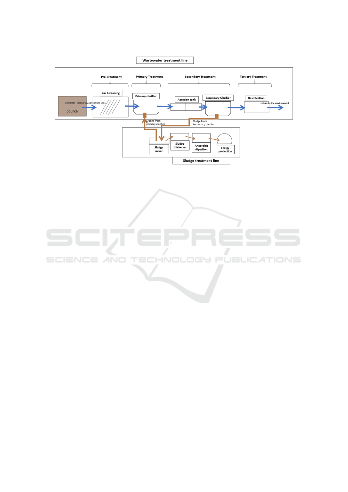
Figure 1: Simpliﬁed scheme of a WWTP operation.

process), the pH value must comply with the emis-

sion limit values considered by the law. According to

the Portuguese Environment Agency ((PAE, 2013)),

these values must be between 5.5 and 9 to be consid-

ered “good”, and between 6.5 and 8.5 to be classiﬁed

as “excellent”.

Over the years, several studies were carried out

addressing the related topics, air, and water quality.

Literature shows some researches addressing the UV

index forecast. It stands out the using of a CART

regression model in the presence of several environ-

mental conditions. This study shows that when ob-

served opacity are generated better predictions com-

pared to using clear-sky UV ((Burrows, 1997)). Fur-

ther, addressing the atmospheric pollutants, a study

in the city of Hangzhou, in China, was deployed.

This research makes use of Recurrent Neural Net-

work (RNN) and RFs for analysis and accurate fore-

cast of several atmospheric pollutants (including CO),

based on the prediction of the future 24h ((Feng et al.,

2019)). Furthermore, regarding this topic, recent re-

search exposes the use of ML to forecast air quality

in the city of California. Using Support Vector Re-

gression (SVR) was hourly predicted pollutant con-

centrations, like CO, sulfur dioxide, nitrogen dioxide,

ground-level ozone, and particulate matter ((Castelli

et al., 2020)).

Regarding WWTPs, some studies have already

engaged on using a hybrid statistical-ML approach

to forecasting the ammonia presented in the activated

sludge, to improve the control process of WWTPs

((Gawdzik et al., 2016)). Further, a few studies have

already focused on the use of ML models to moni-

tored the WWTPs operations ((Harrou et al., 2018;

Dairi et al., 2019)).

3 MATERIALS AND METHODS

The next lines describe the materials and methods

used in this work, including the used datasets, to

achieve the proposed goals.

3.1 Data Exploration

Two datasets support this research. The ﬁrst con-

cerns the air quality of a Portuguese city, while the

other presents water quality features with respect to a

WWTP within the same city.

The ﬁrst dataset reveals data about the UV index

(UV Value), air pollutants concentration (CO Value

and SO

Value), and weather conditions (Clouds,

Temperature, and Weather Description). It presents

11817 hourly observations in a time range that goes

from 24-07-2018 to 23-03-2020, with some excep-

tions being observed. There are no missing values.

An analysis to the UV Value and the CO Value shows

that, as expected, these data do not present a signiﬁ-

cant variation through a day.

Figure 2 illustrates the mean monthly UV index

behavior in the time range under study. It shows that

this feature presents a well-deﬁned behavior, reveal-

ing that during July it reached the highest value, and

the lowest in December, on average.

Figure 3, on the other hand, shows the CO con-

centration over time, in the deﬁned time interval. The

graph illustrates that higher values are reached in Oc-

tober as well as the presence of missing time steps.

The second dataset contains water quality data

from a real WWTP. The main features are the Dis-

solved Oxygen (DO) (from the anoxic and the aerated

zones), the water pH from the secondary clariﬁer, and

ICAART 2021 - 13th International Conference on Agents and Artiﬁcial Intelligence

1212

Figure 2: Average UV index per

month.

Figure 3: CO concentration over time. Figure 4: pH in the tertiary treatment

unit over time.

the temperature from the tertiary treatment unit. This

dataset presents a total of 2379 observations deﬁned

in a time range that goes from 2016-01-01 to 2020-

05-28. These dataset presents missing values.

Figure 4 illustrates the pH, in the tertiary treatment

unit, over time. It depicts that the values mostly com-

ply with those deﬁned by the Portuguese Environment

Agency (illustrated by the horizontal lines).

Finally, Table 1 depicts the available features in

both datasets.

Table 1: Features available in both datasets.

Dataset Feature (unit)

Air

Quality

UV Value

CO Value (ppm)

Value (ppm)

Clouds (%)

Temperature (ºC)

Weather Description

Date (YYYY-MM-DD HH:mm:ss)

Water

Quality

DO-Aerated Zone (mg/L)

DO-Anoxic Zone (mg/L)

pH-Secondary Clariﬁer

Temperature-Tertiary Treatment

(ºC)

Date (YYYY-MM-DD HH:mm:ss)

3.2 Data Preparation

With respect to the air quality dataset, the UV Value

and the CO Value (target features) do not present a

signiﬁcant variation during a day. For this reason,

data were grouped by day, using the mean value of

the UV Value, CO Value, SO

Value, Clouds, and the

Temperature. Further, for the nominal feature, the

Weather Description, the most frequent description in

a day was the one used, i.e., the mode. It resulted in a

dataset made by 506 daily observations. Furthermore,

since neural networks only accept numerical features

as inputs, the Weather Description was labeled en-

coded. Date ﬁelds were also extracted, creating three

new features: day, month, and year in regard to each

observation.

With respect to the water quality dataset, the main

transformations focused on handling the missing val-

ues. Most of these were computed through linear

interpolation, and when that was not possible, the

records were removed. After this process, the dataset

was left with 2149 observations. Date ﬁelds were

also extracted, creating four new features: hour, day,

month, and year in regard to each observation.

This research was originally a regression problem

due to the nature of the target features. It was settled,

however, that it might be of interest to explore the pre-

diction of the UV Value as a classiﬁcation problem as

well. This feature was converted into different levels,

those established by the World Health Organization

(WHO), through the creation of four bins: Low (when

the UV index was between 0 and 2), Medium (UV in-

dex between 3 and 5), High (UV index between 6 and

7), and Very High (UV index higher than 8). No in-

dexes higher than 11 were found in the dataset.

3.3 Technologies

The technologies used to develop this research were

the KNIME software as well as Python, supported

by Keras and TensorFlow as main APIs. Besides,

other important libraries such as pandas, matplotlib,

NumPy, and scikit-learn were also used. To tune and

train the deep learning models the Google Colabo-

ratory cloud service was used. This service uses a

Jupyter notebook environment and runs totally in the

cloud, using GPUs.

4 EXPERIMENTS

After preparing the data, multiple scenarios were cre-

ated to study the impact of each feature in the models’

performance.

Using Machine Learning to Forecast Air and Water Quality

1213

4.1 UV Index Scenarios

First, for the UV index forecasting, ﬁve scenarios

were built, representing a gradual increase in the fea-

tures that constituted them. Thereby, the scenarios

were as follows:

1. The ﬁrst scenario has in its constitution the Date,

the CO Value, and the SO

Value, in order to un-

derstand the impact of the atmospheric pollutants;

2. Scenario number two adds the Temperature to the

previous one. Thus, it enables us to understand the

impact of this feature in the outcomes regarding

the UV index prediction;

3. The third scenario adds the Clouds percentage to

the preceding, allowing us to know the inﬂuence

of clouds percentage in the prediction of the UV

index;

4. Scenario number four adds the month to the pre-

vious one, as the data shows that the UV in-

dex has a well-deﬁned behavior according to the

month of the year (higher in the summer months

and smaller in the winter, in the Northern Hemi-

sphere);

5. Scenario number ﬁve adds the Weather descrip-

tion to the prior, to perceive its impact on the mod-

els’ outcomes.

The scenarios described above are used to tune and

evaluate all tree-based models. To train the MLP

model, the same scenarios were used except for the

Date feature, which was replaced by the day, month,

and year. Therefore, scenario number four becomes

useless in this context.

The UV index was also framed as a time series

problem. In this context, LSTM models were con-

ceived and tuned using only the UV Value feature

(framed as a uni-variate problem).

4.2 CO Concentration Scenario

The CO air concentration forecast was exclusively

formulated as a time series problem, with a LSTM

model being conceived and tuned for a single feature,

the CO Value. This is the only scenario created for the

CO air concentration.

4.3 Water pH Scenarios

For water pH forecasting, four scenarios were created,

as follows:

1. Scenario number one is constituted by the Date,

the pH-Secondary clariﬁer, the DO-Aerated Zone,

the DO-Anoxic Zone, and the Temperature-

Tertiary Treatment. This scenario uses all the fea-

tures available from the water quality dataset;

2. Scenario number two excludes the temperature

feature from the previous one, allowing us to un-

derstand the impact of this feature in the water pH

prediction;

3. The third scenario is constituted by the Date, the

DO-Aerated Zone, the DO-Anoxic Zone and the

Temperature-Tertiary Treatment. When compared

with the preceding, this one replaces the pH from

the secondary clariﬁer by the temperate, previ-

ously withdrawn;

4. Scenario number four is constituted by the Date,

the pH-Secondary clariﬁer, and the Temperature-

Tertiary Treatment. It excludes both dissolved

oxygen features to understand its impact on the

forecasts’ quality.

The above scenarios are used to train all tree-based

models. For the MLPs, the date feature is replaced by

four features, i.e., hour, day, month, and year.

4.4 Hyperparameters Searching Space

After building the feature scenarios, the models’ hy-

perparameters were set. Table 2 shows the search-

ing space considered for each hyperparameter of each

model.

5 RESULTS AND DISCUSSION

The best outcomes for each scenario, considering the

optimal hyperparameter combination, are presented

in the next lines. The used evaluation metrics are the

Accuracy and the Mean Absolute Error (MAE).

5.1 UV Index Forecasting

When considering the UV index as a classiﬁcation

problem, the levels deﬁned by WHO were the ones

used to set the target feature as Low, Medium, High,

and Very High. Table 3 presents the results generated

from this process for each model type.

The best candidate model achieved an accuracy

value of 93.5%. It is generated by the MLP model,

making use of the scenario constituted by the atmo-

spheric pollutants and the date ﬁelds as features (Sce-

nario 1). It may indicate that, for the MLP classiﬁca-

tion problem, using the fewest features generate bet-

ter results in this context. Further, for the tree-based

models, Scenario 4 shows the best outcomes, which

ICAART 2021 - 13th International Conference on Agents and Artiﬁcial Intelligence

1214

Table 2: Hyperparameters tested for each model.

Model Hyperparameter Search Space

Decision Tree

Classiﬁcation

Quality measure [Gini Index, Gain ratio]

Pruning method [No pruning, MDL]

Reduced error pruning [True, False]

Minimum records per node From 1 to 15*

Regression

Missing value handling [XGBoost, Surrogate]

Limit number of levels From 1 to 20*

Min. node size From 1 to 15*

Random Forest

Classiﬁcation

Split criterion [Information Gain (Ratio), Gini index]

Tree depth From 1 to 25*

Minimum child node size From 1 to 15*

Number of Models From 100 to 1200**

Regression

Tree depth From 1 to 15*

Minimum child node size From 1 to 15*

Number of Models From 100 to 1200**

MLPs & LSTMs

Activation Function [relu, tanh, sigmoid]

Hidden Layers [1, 2, 3]

Learn Rate [0.001, 0.005, 0.01]

Neurons [16, 32, 64, 128]

Batch Size [16, 23, 30]

Time steps*** [7, 14, 21]

* With a step size of 1

** With a step size of 100

*** LSTM hyperparameter

Table 3: Accuracy values, per scenario, for the classiﬁcation

of the UV index.

Scenario DT RF MLP

1 87.8% 79.6% 93.5%

2 77.9% 83.8% 91.1%

3 74.9% 82.2% 90.5%

4 92.1% 91.5% -

5 89.5% 91.3% 89.3%

proves that using the month name as a feature results

in the best accuracy.

DTs show their best performance (Scenario 4) us-

ing the Gini Index as the quality measure, no pruning,

and a minimum child node size of 2. Regarding this

model, were perceived that for all the scenarios, no

pruning revealed to be the best choice. It produces

better results, probably due to the low complexity of

the generated trees. So, all the branches are consid-

ered signiﬁcant, and its removal leads to a decrease

in the model’s performance. For the RFs, the best

outcomes (again, Scenario 4) are generated using In-

formation Gain Ratio as quality measure, a tree depth

of 14, a minimum child node of 9, and a number of

models equal to 500, i.e., the number of trees to be

learned. Since the maximum number that was experi-

mented was 1200, the best outcome generated by this

model is produced with a medium level of complex-

ity. For the MLPs, the best candidate used 3 hidden

layers, a learning rate of 0.001, 64 neurons per layer,

a batch size of 23, and ’relu’ as activation function.

When considering the UV index as a regression

problem, the results are the ones presented in Table 4.

For the tree-based models, the best scenario is, again,

Scenario 4, which adds the month name to its con-

stitution. Further, for the MLP model, the best result

arises from Scenario 5. It shows that, regarding this

particular model, a higher amount of features gener-

ates the best outcome. Overall, the best model is a DT

with a MAE of just 0.37.

Table 4: MAE values, per scenario, regarding UV Index

forecasting.

Scenario DT RF MLP

1 0.589 1.438 0.490

2 0.789 0.739 0.514

3 0.901 1.128 0.521

4 0.373 0.410 -

5 0.433 1.598 0.452

For the DTs, the best performance (Scenario 4)

uses XGBoost to handle missing values, a tree depth

of 6, and a minimum node size of 5. For the RFs, the

best performance (Scenario 4) shows a tree depth of

11, a minimum child node size of 1, and a number

of models equal to 1000, a high value that shows the

need for a more complex model. For the MLP, the

best candidate used ’relu’ as the activation function, 2

hidden layers, a learning rate of 0.001, 32 neurons per

layer, and a batch size of 16 (Scenario 5).

Finally, the last approach concerns the UV index

Using Machine Learning to Forecast Air and Water Quality

1215

as a time series problem. For this, LSTM models were

conceived, making recursive multi-step forecasts, i.e.,

the goal was to forecast the next three days. The

best LSTM candidate achieved an overall MAE of just

0.151, clearly outperforming the results obtained pre-

viously, with MLPs and the tree-based models. The

hyperparameter combination producing the best can-

didate makes use of the ’tanh’ as activation function,

a single hidden layer, a learning rate of 0.01, 16 neu-

rons per layer, and a batch size of 16 sequences. Fur-

ther, it uses 21 time steps to create a single sequence,

i.e., it uses the last three weeks to forecast the next

three days. Even though the best candidate does not

have a complex architecture, it still took a consider-

able amount of time to train, especially when com-

pared to the tree-based models.

5.2 CO Concentration Forecasting

The CO is one of the primary pollutants. Hence, in

this research, the air concentration of this pollutant

was set only as a time series problem. The same logic

that was used to forecast the UV index is applied to

the CO concentration, with the best LSTM candidate

reaching a MAE of 1.345×10

−7

. The best hyperpa-

rameter combination uses a single layer, ’relu’ as ac-

tivation function, a learning rate of 0.005, 16 neurons,

and a batch size of 16. Moreover, using a sequence

of three weeks (in which the predictions are based)

shows to be the best option, i.e., time steps equal to

21. It indicates a simple model, taking into account

the maximum tested values. However, it also takes a

long time to run, as aforementioned.

5.3 Water pH Forecasting

The water pH is part of a WWTP, in particular, to its

tertiary phase, i.e., the moment right before the wa-

ter is discharged back to natural sources. This fore-

cast arises in order to try to mitigate the environmen-

tal consequences of these systems concerning water

quality.

Table 5: MAE values, per scenario, for water pH forecast-

ing.

Scenario DT RF MLP

1 0.106 0.114 0.119

2 0.184 0.180 0.146

3 0.195 0.193 0.154

4 0.106 0.120 0.118

By evaluating Table 5, one may conclude that all

the best candidate models produce very similar re-

sults, even though from different scenarios. The best

DT uses, as features, the pH from the secondary clari-

ﬁer, the temperature, and the date (Scenario 4). How-

ever, it shows very similar outcomes when compared

with Scenario 1, which adds, as new features, the dis-

solved oxygen from the aerated and the anoxic zones.

Further, these two scenarios are also the ones depict-

ing the best solutions for the best RF and the best

MLP candidates. So, it is possible to conclude that,

when used together, the temperature and the pH from

the secondary clariﬁer are important features to fore-

cast the pH of the water from the tertiary treatment

unit. The dissolved oxygen features, by themselves,

do not seem to be a decent approach to predict water

pH.

The best candidate DT presents its best perfor-

mance (Scenario 4) using the surrogate as missing

value handling, a tree depth of 5, and a minimum

node size of 5. The best RF shows its best outcome

(Scenario 1) using a tree depth of 4, a minimum child

node size of 8, and 500 models, exhibiting a medium

complexity. On the other hand, the best MLP model

(Scenario 4) is constituted by 64 neurons per layer,

three hidden layers, a learning rate of 0.005, and a

batch size of 16. Again, this model took longer to

train when compared to the tree-based models.

6 CONCLUSIONS AND FUTURE

WORK

Environmental sustainability is a big concern for en-

tities nowadays. The detrimental effects on public

health, ecosystem imbalance, and climate changes are

increasingly evident. Thus, this research conceived

and tune several supervised ML models, with dif-

ferent degrees of complexity, to multiple several pa-

rameters in the environmental sustainability domain.

Regarding the air quality and atmospheric pollution,

both the UV index and the CO air concentration were

addressed. For the UV index forecast, when treating

it as a classiﬁcation problem, an accuracy of approxi-

mately 93% was achieved. In addition, predicting it as

a regression problem resulted in a MAE of 0.37 units.

For both approaches, the used features proved to be

relevant in the quality of the forecasts. Moreover, the

UV index was set as a time series problem using a

LSTM model. The best candidate model achieved

a MAE of 0.15, using a uni-variate approach. With

regard to the CO air concentration, a MAE value

of 1.345×10

−7

was achieved, being possible to con-

clude that it is likely to predict these parameters with

small errors, using simple or more complex models.

The water pH was also predicted, achieving a

MAE of, approximately, 0.11 units, with the DTs,

ICAART 2021 - 13th International Conference on Agents and Artiﬁcial Intelligence

1216

RFs and MLPs revealing themselves capable of pro-

ducing accurate forecasts. Furthermore, the used fea-

tures revealed themselves to have a signiﬁcant impact

on the outcomes.

This research shows that it is possible to antici-

pate problematic situations and reduce their negative

impacts, with satisfactory accuracy. As future work,

the goal is to forecast the CO air concentration using

additional models, as well as distinct attributes. Ad-

ditionally, a major goal focuses on forecasting more

parameters related to Environmental Sustainability, in

order to promote a more sustainable and green soci-

ety.

ACKNOWLEDGEMENTS

This work was supported by National Funds through

the Portuguese funding agency, FCT - Founda-

tion for Science and Technology, within the project

DSAIPA/AI/0099/2019. The work of Bruno Fernan-

des is also supported by a Portuguese doctoral grant,

SFRH/BD/130125/2017, issued by FCT in Portugal.

REFERENCES

Block, M. L., Elder, A., Auten, R. L., Bilbo, S. D., Chen,

H., Chen, J. C., Cory-Slechta, D. A., Costa, D., Diaz-

Sanchez, D., Dorman, D. C., Gold, D. R., Gray, K.,

Jeng, H. A., Kaufman, J. D., Kleinman, M. T., Kir-

shner, A., Lawler, C., Miller, D. S., Nadadur, S. S.,

Ritz, B., Semmens, E. O., Tonelli, L. H., Veronesi, B.,

Wright, R. O., and Wright, R. J. (2012). The outdoor

air pollution and brain health workshop. NeuroToxi-

cology, 33(5):972–984.

Burrows, W. (1997). Cart regression models for predict-

ing uv radiation at the ground in the presence of cloud

and other environmental factors. Journal of Applied

Meteorology, 36(5):531–544. cited By 48.

Castelli, M., Clemente, F., Popovi

c, A., Silva, S., and Van-

neschi, L. (2020). A machine learning approach to

predict air quality in california. Complexity, 2020.

cited By 0.

Cohen, A. J., Brauer, M., Burnett, R., Anderson, H. R.,

Frostad, J., Estep, K., Balakrishnan, K., Brunekreef,

B., Dandona, L., Dandona, R., Feigin, V., Freedman,

G., Hubbell, B., Jobling, A., Kan, H., Knibbs, L., Liu,

Y., Martin, R., Morawska, L., Pope, C. A., Shin, H.,

Straif, K., Shaddick, G., Thomas, M., van Dingenen,

R., van Donkelaar, A., Vos, T., Murray, C. J., and

Forouzanfar, M. H. (2017). Estimates and 25-year

trends of the global burden of disease attributable to

ambient air pollution: an analysis of data from the

Global Burden of Diseases Study 2015. The Lancet,

389(10082):1907–1918.

Dairi, A., Cheng, T., Harrou, F., Sun, Y., and Leiknes, T.

(2019). Deep learning approach for sustainable wwtp

operation: A case study on data-driven inﬂuent condi-

tions monitoring. Sustainable Cities and Society, 50.

cited By 2.

Feng, R., Zheng, H.-J., Gao, H., Zhang, A.-R., Huang, C.,

Zhang, J.-X., Luo, K., and Fan, J.-R. (2019). Recur-

rent neural network and random forest for analysis and

accurate forecast of atmospheric pollutants: A case

study in hangzhou, china. Journal of Cleaner Produc-

tion, 231:1005–1015. cited By 20.

Gawdzik, J., Szelag, B., Bezak-Mazur, E., and Stoinska,

R. (2016). Application of selected nonlinear meth-

ods to forecast the amount of excess sludge. Rocznik

Ochrona Srodowiska, 18(2):695–708.

Harrou, F., Dairi, A., Sun, Y., and Senouci, M. (2018).

Wastewater treatment plant monitoring via a deep

learning approach. volume 2018-February, pages

1544–1548. cited By 2.

Hino, M., Benami, E., and Brooks, N. (2018). Machine

learning for environmental monitoring. Nature Sus-

tainability, 1(10):583–588.

Igoe, D., Parisi, A., and Carter, B. (2013). Characterization

of a Smartphone Camera’s Response to Ultraviolet A

Radiation. International Journal of Remote Sensing,

pages 215–218.

Isabel Molina-G

omez, N., Rodr

ıguez-Rojas, K., Calder

on-

Rivera, D., Luis D

ıaz-Ar

evalo, J., and L

opez-Jim

enez,

P. A. (2020). Using machine learning tools to clas-

sify sustainability levels in the development of urban

ecosystems. Sustainability (Switzerland), 12(8).

Lee, K. K., Spath, N., Miller, M. R., Mills, N. L., and

Shah, A. S. (2020). Short-term exposure to carbon

monoxide and myocardial infarction: A systematic re-

view and meta-analysis. Environment International,

143(June):105901.

Norval, M., Lucas, R. M., Cullen, A., de Gruijl, F.,

Longstreth, J., Takizawa f, Y., and van der Leung, J.

(2011). The human health effects of ozone depletion

and interactions with climate change. Photochemical

and Photobiological Sciences, 10(2):173.

PAE (2013). https://www.apambiente.pt/. Accessed: 2020-

10-01.

Qiu, J., Wu, Q., Ding, G., Xu, Y., and Feng, S. (2016). A

survey of machine learning for big data processing.

Eurasip Journal on Advances in Signal Processing,

2016(1).

Sandryhaila, A. and Moura, J. M. (2014). Representa-

tion and processing of massive data sets with irregular

structure. IEEE SIGNAL PROCESSING MAGAZINE,

5(31):80–90.

Sarkodie, S. A. (2021). Environmental performance, bio-

capacity, carbon & ecological footprint of nations:

Drivers, trends and mitigation options. Science of the

Total Environment, 751:141912.

Spellman, F. R. (2013). Handbook of Water and Wastewater

Treatment Plant Operations.

Using Machine Learning to Forecast Air and Water Quality

1217