An Ensemble-based Approach by Fine-Tuning the Deep Transfer

Learning Models to Classify Pneumonia from Chest X-Ray Images

Sagar Kora Venu

Department of Analytics, Harrisburg University of Science and Technology, Harrisburg, PA 17101, U.S.A.

Keywords:

Pneumonia Classiﬁcation, Deep Learning, Transfer Learning, Chest X-Ray, Medical Imaging, Computer

Vision.

Abstract:

Pneumonia is caused by viruses, bacteria, or fungi that infect the lungs, which, if not diagnosed and treated in

time, can be fatal and lead to respiratory failure. More than 250,000 individuals in the United States, mainly

adults, are diagnosed with pneumonia each year, and 50,000 die from the disease. Chest Radiography (X-ray)

is widely used by radiologists to detect pneumonia. It is not uncommon to overlook pneumonia detection for

a well-trained radiologist, which triggers the need for improvement in the accuracy of the diagnosis. There-

fore, we propose using transfer learning, which can reduce the neural network’s training time and minimize

the generalization error to improve the accuracy of the diagnosis. We trained, ﬁne-tuned the state-of-the-art

deep learning models such as InceptionResNet, MobileNetV2, Xception, DenseNet201, and ResNet152V2 to

classify pneumonia accurately. Later, we created a weighted average ensemble of these models and achieved

a test accuracy of 98.46%, precision of 98.38%, recall of 99.53%, and f1 score of 98.96%. These performance

metrics of accuracy, precision, and f1 score are at their highest levels ever reported in the literature, which can

be considered a benchmark for the accurate pneumonia classiﬁcation.

1 INTRODUCTION

Pneumonia is an acute respiratory infection caused

by bacteria, fungi, or viruses with mild to life-

threatening conditions that, if not diagnosed, can

lead to respiratory failure (Pne, a), (Pne, b). More

than 250,000 individuals in the United States, mainly

adults, are diagnosed with pneumonia each year,

50,000 die from the disease (Pne, b). Pneumonia is

also the world’s largest infectious cause of child mor-

tality, accounting for 15% of all infant deaths under

ﬁve years of age (Pne, a). Standard tests for pneumo-

nia diagnosis include blood tests, chest X-rays, pulse

oximetry, sputum tests, arterial blood gas tests, bron-

choscopy, pleural ﬂuid culture, and CT scans (Pne,

c). However, chest X-rays are a gold standard tool for

diagnosing pneumonia that can distinguish pneumo-

nia from other respiratory infections (Mandell et al.,

2007). It is not uncommon to overlook pneumonia

detection for a well-trained radiologist, which triggers

the need for improvement in the diagnosis’s accuracy.

Deep learning is now the state-of-the-art paradigm

of machine learning, leading to enhanced perfor-

https://orcid.org/0000-0002-5035-1605

mance in various areas, including medical image clas-

siﬁcation, natural language processing, object detec-

tion, segmentation, and other tasks (Litjens et al.,

2017), (Shen et al., 2017), (Lundervold and Lunder-

vold, 2019). In particular, the deep Convolutional

Neural Nets (CNN), which almost halve the error

rate in the competition for Object Recognition - the

Imagenet Large Scale Visual Recognition Competi-

tion (ILSVRC), have been highly dominant in ﬁeld of

computer vision (Krizhevsky et al., 2012). Follow-

ing CNN’s success with computer vision, the med-

ical image analysis community started to recognize

the potential of deep learning techniques to achieve

an expert level of performance in classiﬁcation, seg-

mentation, and detection of medical images (Litjens

et al., 2017). This work’s signiﬁcant contribution is

that we propose the weighted average ensemble-based

approach by ﬁne-tuning the deep transfer learning

models (InceptionResNet, MobileNetV2, Xception,

DenseNet201, ResNet152V2) to improve the deep

learning classiﬁcation model’s performance metrics.

390

Kora Venu, S.

An Ensemble-based Approach by Fine-Tuning the Deep Transfer Learning Models to Classify Pneumonia from Chest X-Ray Images.

DOI: 10.5220/0010377403900401

In Proceedings of the 13th International Conference on Agents and Artiﬁcial Intelligence (ICAART 2021) - Volume 2, pages 390-401

ISBN: 978-989-758-484-8

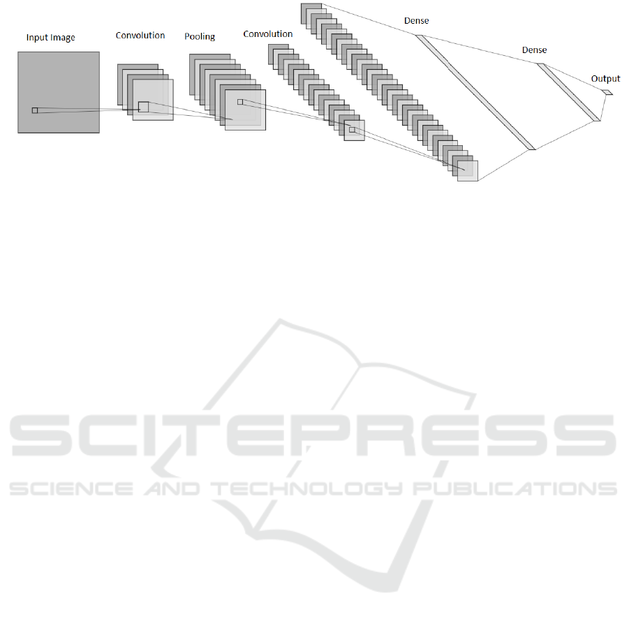
Figure 1: CNN Architecture.

2 RELATED WORK

The deep learning framework proposed by (Liang

and Zheng, 2020) incorporates transfer learning com-

bined with residual thought and dilated convolution

for the classiﬁcation of pediatric pneumonia images,

achieved a test recall of 96.7%, and an f1 score of

92.7%. To classify pneumonia from chest X-ray

images, (Chouhan et al., 2020) and (Hashmi et al.,

2020) used transfer learning and proposed an en-

semble model that combined the pre-trained models’

results, achieving 96.4% accuracy and 98.43% ac-

curacy respectively from the unseen dataset of the

Guangzhou Women and Children’s Medical Center.

(Stephen et al., 2019) trained a convolutional neural

network from scratch to detect the presence of pneu-

monia from a series of chest X-ray images resulting

in approximately 94% validation accuracy. (Rahman

et al., 2020) used transfer learning from DenseNet201

architecture, a pre-trained deep convolutional net-

work on the Imagenet dataset, and reported a 98% ac-

curacy of pneumonia classiﬁcation. (Ayan and

Unver,

2019) used Xception and Vgg16 as transfer learn-

ing models and compared the accuracy between them

only to report the accuracy of the Xception network

exceeds the Vgg16 network at 87% and 82%.

This paper’s signiﬁcant contribution is using a

weighted average ensemble method by ﬁne-tuning the

state-of-the-art pre-trained neural networks trained on

the Imagenet dataset to achieve the best classiﬁcation

performance metrics ever published in the literature.

3 METHODS AND MATERIALS

Convolutional Neural Networks are a type of deep

learning models designed for processing data in the

form of multiple arrays, e.g., a color image has three

channels (RGB), each channel consists of 2D arrays

containing pixel intensities (LeCun et al., 2015). The

architecture of typical Convolutional Neural Network

is shown in Figure 1.

The ﬁrst few stages in the architecture are a series

of convolution layers and pooling layers. The image

is fed as an input to the convolution layer to extract

meaningful features (feature maps). A non-linearity

is applied to the feature maps, followed by a pooling

layer that merges similar features into one by com-

puting either the maximum or average value for each

patch on the feature map, which typically reduces the

representation’s dimensions. The output from the last

stage of the convolution layer, non-linearity, and pool-

ing layer is subjected to fully-connected layers, fol-

lowed by a softmax to output the predictions.

3.1 Transfer Learning

Machine learning algorithms assume that training and

test data will come from the same distribution and fea-

ture space (Pan and Yang, 2009). It may not hold good

in real-world applications, particularly in the ﬁeld of

medical imaging, where obtaining a huge amount of

training data is itself a major bottleneck due to high

annotation costs and the protection of patients’ pri-

vacy. Transfer Learning, which is a technique that

improves the learning in a new domain through the

transfer of knowledge from a related domain (Weiss

et al., 2016), (Torrey and Shavlik, 2010), bypasses

the assumption that the training data must be inde-

pendent and identically distributed (i.i.d) with the test

data (Tan et al., 2018).

3.2 Pre-trained Image Classiﬁcation

Models

Pre-trained models are the models trained on large

benchmark datasets, where the models have already

learned to extract a wide variety of features, can be

An Ensemble-based Approach by Fine-Tuning the Deep Transfer Learning Models to Classify Pneumonia from Chest X-Ray Images

391

Input Image: 299 x 299 x 3

Conv 32, 3 x 3, stride 2, ReLu

Conv 64, 3 x 3, ReLu

SeparableConv 128, 3 x 3

ReLu, SeparableConv 128, 3 x 3

MaxPooling 3 x 3, stride 2

ReLu, SeparableConv 256, 3 x 3

MaxPooling 3 x 3, stride 2

ReLu, SeparableConv 256, 3 x 3

MaxPooling 3 x 3, stride 2

Conv 1 x 1

Stride 2

Conv 1 x 1

Stride 2

Conv 1 x 1

Stride 2

19 x 19 x 728 feature maps

Entry Flow

ReLu, SeparableConv 728, 3 x 3

19 x 19 x 728 feature maps

Repeated 8 times

ReLu, SeparableConv 728, 3 x 3

ReLu, SeparableConv 1024, 3 x 3

MaxPooling 3 x 3, stride 2

SeparableConv 1536, 3 x 3, ReLu

SeparableConv 2048, 3 x 3, ReLu

GlobalAveragePooling, 2048

Conv 1 x 1

Stride 2

Softmax, 1000

Middle Flow

Exit Flow

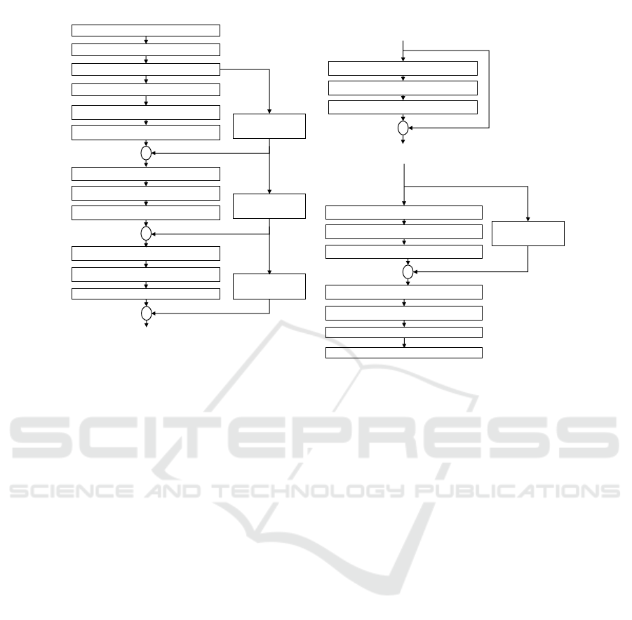
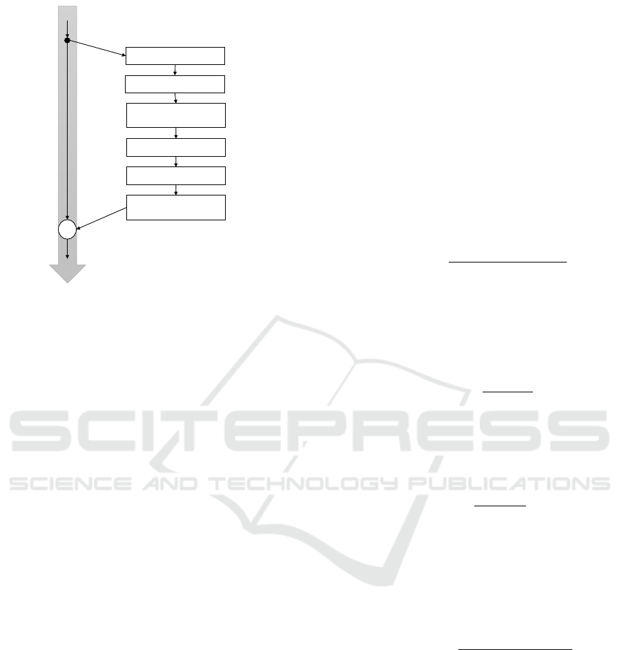
Figure 2: Xception Architecture.

used as a starting point to learn on a new task in a

related domain. It is a common practice in the ﬁeld

of computer vision to use transfer learning via pre-

trained models. In the following sub-sections, we will

brieﬂy introduce the pre-trained models used in this

study.

3.2.1 Xception

Xception is one of the state-of-the-art deep learn-

ing model architectures, based on depthwise separa-

ble convolution layers developed by Chollet (Chol-

let, 2017) from Google Inc, which is also known as

the extreme version of Inception. The depthwise sep-

arable convolution consists of a depthwise convolu-

tion - a spacial convolution performed independently

across every input channel, followed by a pointwise

convolution - a 1 x 1 convolution that changes the in-

put dimensions. But the extreme form of the incep-

tion module consists of a pointwise convolution fol-

lowed by a depthwise convolution, and another dif-

ference among them is the presence/ absence of the

non-linearity layer. Usually, depthwise separable con-

volutions are implemented without non-linearities be-

tween a depthwise convolution and pointwise convo-

lution. In the extreme version of the inception mod-

ule, depthwise convolution and pointwise convolution

are followed by a ReLU non-linearity.

The Xception architecture is shown in Figure 2,

which is divided into three major phases: Entry ﬂow,

Middle Flow, and Exit ﬂow. There are 36 convolu-

tion layers in the architecture that are structured into

14 modules. Except for the ﬁrst and last modules,

all other modules have linear residual connections

around them. In other words, Xception architecture

is a linear stack of depthwise separable convolutions

with residual connections, when trained on ImageNet

dataset (Russakovsky et al., 2015), Chollet (Chollet,

2017) reported a top-1 accuracy of 79.0% and top-5

accuracy of 94.5%.

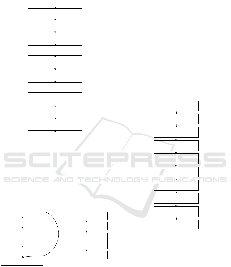
3.2.2 MobileNetV2

(Sandler et al., 2018) have introduced a neural net-

work architecture designed speciﬁcally for mobile

and resource-intensive environments. They intro-

duced a unique layer module known as the inverted

residual with a linear bottleneck, which takes a low di-

mensional compressed representation as an input that

is then expanded to a high dimension and later ﬁl-

tered with a lightweight depth-wise convolution. The

MobileNet-V2 architecture is shown in Figure 3 that

contains an initial fully convolutional layer followed

by residual bottleneck layers.

There are two types of blocks in the network, as

shown in Figure 4: one is the residual block of stride

1, and another is a block with stride 2 for downsiz-

ing the input from the previous layer. Each block has

three layers: The ﬁrst layer is a 1 x 1 Convolution

with ReLu6 activation, the second layer is a depth-

ICAART 2021 - 13th International Conference on Agents and Artiﬁcial Intelligence

392

Input Image: 224 x 224 x 3

1 x Conv2D: stride 2

Output size : 112 x 112 x 32

1 x Bottleneck: Stride 1

Output Size: 112 x 112 x 16

2 x Bottleneck: Stride 2

Output Size: 56 x 56 x 24

3 x Bottleneck: Stride 2

Output Size: 28 x 28 x 32

4 x Bottleneck: Stride 2

Output Size: 14 x 14 x 64

3 x Bottleneck: Stride 1

Output Size: 14 x 14 x 96

Global Average Pooling

Output: 1280

Softmax

Output: 1000

3 x Bottleneck: Stride 2

Output Size: 7 x 7 x 160

1 x Bottleneck: Stride 1

Output Size: 7 x 7 x 320

1 x Conv2D: stride 1

Output size : 7 x 7 x 1280

Figure 3: MobileNet-V2 Architecture.

wise convolution, which is responsible for perform-

ing lightweight ﬁltering by applying a single convolu-

tional ﬁlter per input channel, and the third layer is a

1 x 1 Convolution, which is also referred to as a point-

wise convolution that creates new features through

computing linear combinations of the input channels.

Input

Conv 1 x 1, ReLu6

Depth-wise

Convolution 3 x 3,

ReLu6

Conv 1 x 1, Linear

Add

Stride=1 Block

Input

Conv 1 x 1, ReLu6

Depth-wise

Convolution 3 x 3,

Stride=2, ReLu6

Conv 1 x 1, Linear

Stride=2 Block

Figure 4: MobileNet-V2 Bottleneck Stride Blocks.

With this architecture, (Sandler et al., 2018)

trained a neural network model on the ImageNet

dataset (Russakovsky et al., 2015) and compared the

performance with other similar mobile models: Shuf-

ﬂeNet and NasNet-A, and reported a top-1 accuracy

of 74.7% with ShufﬂeNet at 73.7% and NasNet-A at

74.0%.

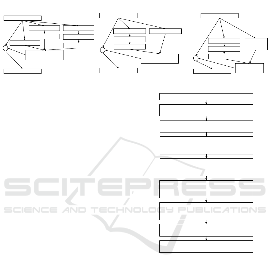
3.2.3 InceptionResNetV2

(Szegedy et al., 2016a) studied the combination of

Inception architecture (Szegedy et al., 2016b) and

Residual connections (He et al., 2016a), and proposed

an architecture that is based on the Inception family of

architectures by replacing the inception module with

a hybrid Inception-ResNet module as shown in Fig-

ure 6, which are three variants: 1. Inception-ResNet-

A for 35 x 35 grid, 2. Inception-ResNet-B for 17 x

17 grid, and 3. Inception-ResNet-C for 8 x 8 grid.

(Szegedy et al., 2016a) argued that training with resid-

ual connections signiﬁcantly accelerated the training

of Inception networks. The large scale schema struc-

ture and the detailed structure of its components are

shown in Figure 5.

Input Image

299 x 299 x 3

Stem

Output: 35 x 35 x 256

5 x Inception-resnet-A

Output: 35 x 35 x 256

Reduction-A

Output: 17 x 17 x 896

10 x Inception-resnet-B

Output: 17 x 17 x 896

Reduction-B

Output: 8 x 8 x 1792

5 x Inception-resnet-C

Output: 8 x 8 x 1792

Average Pooling

Output: 1792

Dropout (keep 0.8)

Output: 1792

Softmax

Output: 1000

Figure 5: InceptionResNetV2 - Large scale schema struc-

ture.

The input image of size 299 x 299 x 3 under-goes

a series of convolutions in the Stem module, followed

by the hybrid Inception-ResNet modules. Each hy-

brid Inception-ResNet module is followed by a Re-

duction module to reduce the dimensions of the rep-

resentation.

Later, the ﬁnal hybrid Inception-ResNet mod-

ule’s output is fed to the average pooling layer, fol-

lowed by a dropout layer to output the predictions.

The design of such deep neural networks that in-

creases the number of layers leads to instability dur-

ing training. The network may die early, for exam-

ple. (Szegedy et al., 2016a) suggested scaling down

An Ensemble-based Approach by Fine-Tuning the Deep Transfer Learning Models to Classify Pneumonia from Chest X-Ray Images

393

Schema for

Inception-ResNet-A

RELU activation

1x1 Conv (32)

1x1 Conv (32) 1x1 Conv (32)

3x3 Conv (32)

3x3 Conv (48)

3x3 Conv (64)

1x1 Conv

(384 Linear)

RELU activation

1x1 Conv (128) 1x1 Conv (192)

1x7 Conv (160)

7x1 Conv (192)

1x1 Conv

(1154 Linear)

RELU activation

Schema for

Inception-ResNet-B

Schema for

Inception-ResNet-C

RELU activation

1x1 Conv (192)

1x1 Conv

(192)

1x3 Conv (224)

3x1 Conv (256)

1x1 Conv

(2048 Linear)

RELU activation

Figure 6: Schema for Inception-ResNet modules.

the residuals before adding them to the previous ac-

tivation layer to stabilize the training, and (He et al.,

2016a) suggested a two-phase training where the ﬁrst

warm-up phase is performed with a low learning rate

and followed by a high learning rate in the second

phase. (Szegedy et al., 2016a) also trained an ensem-

ble of one Inception-v4 and three Inception-ResNet-

v2 models on the ILSVRC 2012 classiﬁcation task

(ImageNet dataset (Russakovsky et al., 2015)) and

achieved 3.08% top-5 error rate on the test set of the

ImageNet dataset.

3.2.4 ResNet152V2

The Deep Residual Networks introduced by (He et al.,

2016a) have improved the accuracy of the deep archi-

tecture models and are shown to have excellent con-

vergence behaviors. (He et al., 2016b) studied the

propagation formulation behind the residual blocks,

i.e., to create a direct path for propagating informa-

tion through the entire network including the residual

unit as shown in Figure 8 and demonstrated that when

the identity maps are used as the skip connections

and after-addition activation, forward and backward

signals are directly propagated between any residual

blocks.

Identity mappings help protect the network from

vanishing gradient problem. The signiﬁcant differ-

ence between ResNet-V1 and ResNet-V2 is that be-

fore the convolution, ResNet-V2 performs batch nor-

malization and ReLU activation at the input; whereas,

ResNet-V1 performs convolution, followed by batch

normalization and ReLU activation. The architecture

of ResNet152-v2 is shown in Figure 7, which takes an

input image of size 224 x 224 x 3 that goes through an

initial convolution with a kernel size of 7 x 7 followed

by a Pooling operation with a kernel size of 3 x 3.

Later, the pooling layer’s output is passed on to a

series of Residual blocks, each containing three lay-

ers: 1 x 1 Convolution, 3 x 3 convolution, and a 1

x 1 convolution, which is then followed by an Av-

erage Pooling layer and a fully connected layer with

Input Image: 224 x 224 x 3

Conv1: Patch 7 x 7, stride 2,

Output size : 112 x 112 x 64

Pool: Patch 3 x 3, Stride 2

Output Size: 56 x 56 x 64

3 x Conv2_x: [(Conv: 1 x 1 , 64),

(Conv: 3 x 3, 64), (Conv 1 x 1, 256)]

Output Size: 28 x 28 x 256

8 x Conv3_x: [(Conv: 1 x 1 , 128),

(Conv: 3 x 3, 128), (Conv 1 x 1, 512)

Output Size: 14 x 14 x 512

36 x Conv4_x: [(Conv: 1 x 1 , 256),

(Conv: 3 x 3, 256), (Conv 1 x 1, 1024)]

Output Size: 7 x 7 x 1024

3 x Conv5_x: [(Conv: 1 x 1 , 512),

(Conv: 3 x 3, 512), (Conv 1 x 1, 2048)]

Output Size: 7 x 7 x 2048

Global Average Pooling

Output: 2048

Softmax

Output: 1000

Figure 7: ResNet152-V2 Architecture.

softmax activation to output the class of Imagenet

dataset. When trained on Imagenet dataset (Rus-

sakovsky et al., 2015) with this architecture, (He et al.,

2016b) reported the top-1 error rate of 21.1% and top-

5 error rate of 5.5%.

3.2.5 DenseNet-201

Computer Vision and Pattern Recognition (CVPR) is

an annual international conference regarded as one

of the ﬁeld’s most important and inﬂuential confer-

ences. Densely Connected Convolutional Networks

(DenseNet) introduced by (Huang et al., 2017) won

the best paper award at the CVPR 2017 conference

(CVP, ), which connects each layer of the network in

a feed-forward manner to every other layer.

ICAART 2021 - 13th International Conference on Agents and Artiﬁcial Intelligence

394

Batch Normalization

ReLu Activation

Weight

(Convolution)

Batch Normalization

ReLu Activation

Weight

(Convolution)

l+1

Figure 8: Residual Unit.

DenseNets have a similar advantage to that of

ResNets (He et al., 2016a), (He et al., 2016b) in solv-

ing the problem of vanishing gradients and several

other beneﬁts, including enhancing the propagation of

features between the layers, facilitating the re-use of

features, and signiﬁcantly reducing the overall learn-

able parameters of the network.

The DenseNet-201 large scale architecture is

shown in Figure 9, which takes an input image of

size 224 x 224 x 3 that goes through an initial con-

volution of kernel size 7 x 7 and stride 2, followed

by a Max pooling operation of kernel size 3 x 3 and

stride 2. Later, the max-pooling output is subjected

to a series of dense blocks and transition layers (four

dense blocks and three transition layers). The dense

block consists of a 1 x 1 convolution followed by a 3

x 3 convolution where each convolution operation is a

sequence of Batch Normalization, ReLU Activation,

and Convolution.

The transition layers have a sequence of 1 x 1 con-

volution followed by an average pooling of 2 x 2.

At the end of the fourth dense block, the global av-

erage pooling is carried out with softmax activation.

(Huang et al., 2017) reported that with only 0.8 mil-

lion parameters (about 1/3 of ResNet parameters), the

DenseNet-201 architecture is able to achieve a com-

parable accuracy of ResNet (He et al., 2016b) with

10.2 million parameters. When trained on the Ima-

geNet dataset (Russakovsky et al., 2015), the top-1

error rate was 22.58%, and the top-5 error rate was

6.34%.

3.3 Classiﬁcation Performance Metrics

Evaluation metrics are critical for accessing the per-

formance of a deep learning classiﬁcation model.

There are different metrics of assessment that are

available for these purposes. However, the standard

metrics reported in the literature for deep learning

classiﬁcation tasks are accuracy, precision, recall, f1

score.

3.3.1 Accuracy

The accuracy of the model is calculated using the

equation 1, which is a ratio of correct predictions to

the total predictions.

Accuracy =

T P + T N

T P + T N + FP + FN

(1)

3.3.2 Precision

The precision of the model summarizes model’s ac-

curacy in terms of the number of samples which were

predicted positive and is given by the equation 2.

Precision =

T P

T P + FP

(2)

3.3.3 Recall

Recall of the model is calculated using the equation 3,

that tells how well the positive class was predicted.

Recall =

T P

T P + FN

(3)

3.3.4 F1 Score

F1 score is the calculation of harmonic mean of preci-

sion and recall of the model and is given by the equa-

tion 4

F1 Score = 2 ∗

Precision ∗ Recall

(Precision + Recall)

(4)

3.3.5 AUC Score

AUC score is the measure of area covered by the re-

ceiver operating characteristics (ROC) curve. For a

perfect classiﬁer, the AUC score is 1.0

3.4 Weighted-Average Ensemble

Classiﬁcation Algorithms based on a single architec-

ture/ model often does not capture entire features in

the data for optimal predictions. The aggregation

of multiple algorithms into an ensemble of models

An Ensemble-based Approach by Fine-Tuning the Deep Transfer Learning Models to Classify Pneumonia from Chest X-Ray Images

395

Input Image: 224 x 224 x 3

7 x 7 conv, stride 2,

Output size : 112 x 112 x 64

3 x 3 max pool, Stride 2

Output Size: 56 x 56 x 64

3 x Dense Block (1): [(Conv: 1 x 1),

(Conv: 3 x 3)]

Output Size: 56 x 56 x 256

Transition Layer (1)

conv: 1 x 1, Output Size: 56 x 56 x 128

Average pool: 2 x 2, Output Size: 28 x 28 x 128

Global Average Pooling

Output: 1920

Softmax

Output: 1000

12 x Dense Block (2): [(Conv: 1 x 1),

(Conv: 3 x 3)]

Output Size: 28 x 28 x 512

Transition Layer (2)

conv: 1 x 1, Output Size: 28 x 28 x 256

Average pool: 2 x 2, Output Size: 14 x 14 x 256

48 x Dense Block (3): [(Conv: 1 x 1),

(Conv: 3 x 3)]

Output Size: 14 x 14 x 1792

Transition Layer (3)

conv: 1 x 1, Output Size: 14 x 14 x 896

Average pool: 2 x 2, Output Size: 7 x 7 x 896

32 x Dense Block (4): [(Conv: 1 x 1),

(Conv: 3 x 3)]

Output Size: 7 x 7 x 1920

Figure 9: DenseNet-201 Architecture.

captures the data’s underlying distribution more pre-

cisely, making better predictions (Shahhosseini et al.,

2019), (Brown et al., 2005), (Dietterich, 2000). The

Figure 11 shows the building blocks of the weighted

average ensemble model.

Each transfer learning model’s output is then mul-

tiplied by a weight and then combined linearly, fol-

lowed by a softmax layer to output predictions. Dur-

ing the training process, the weights are optimized

with the condition that they add up to 1. These op-

timized weights determine the contribution of each

transfer learning model in the ﬁnal prediction.

3.5 Dataset Description

For all the experiments conducted in this study, we

used a Chest X-ray dataset by (Kermany et al., 2018).

The dataset comprises 5,856 chest X-ray images

(1583 images labeled as Normal and 4273 images la-

beled as Pneumonia) taken from children are labeled

either Normal or Pneumonia. The original training

and test sets are heavily imbalanced. So, we initially

combined the dataset with all Normal images in one

folder and all the Pneumonia images in another folder.

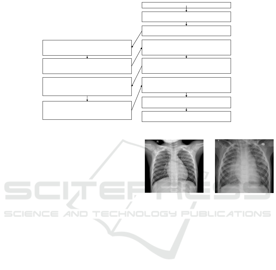
We show a sample of a Normal image and Pneu-

monia image in Figure 10. The dataset was then shuf-

ﬂed and split into training, validation, and test sets, of

which 3,748 images in the training set, 936 images in

the validation set, and 1,172 images in the test set.

3.6 Data Preprocessing

The chest X-ray images in the dataset are in vary-

ing sizes, i.e., all the chest X-ray images’ dimensions

are not the same. However, the deep neural network

(a) Normal Image.

(b) Pneumonia Image.

Figure 10: Sample of a Normal and Pneumonia Image.

architectures utilized in this study as part of transfer

learning expect all the images to be in a common di-

mension. For example, Xception architecture expects

the dimensions of the image (width x height x no. of

Channels) to be 299 x 299 x 3, and width and height

should be no smaller than 71. The dimension of the

input image will also vary by the type of deep neural

network architecture. For example, the DenseNet201

architecture expects the input image shape to be (224

x 224 x 3), with width and height no smaller than

32, and InceptionResNet-V2 expects the input image

shape to be (299 x 299 x 3), with width and height

no smaller than 75. To have common dimensions ac-

cepted by all the architectures used in this study, we

initially resized all the chest X-ray images to have the

shape of (224 x 224 x 3).

Once the images are resized to 224 x 224 x 3,

we created TFRecords of the images and one-hot en-

coded the labels. TFRecord is a binary ﬁle format

that is a standard and the most recommended data

storage format in Tensorﬂow (Use, ). Storing data

in a binary ﬁle format improves the data importing

pipeline’s performance and reduces the model’s train-

ICAART 2021 - 13th International Conference on Agents and Artiﬁcial Intelligence

396

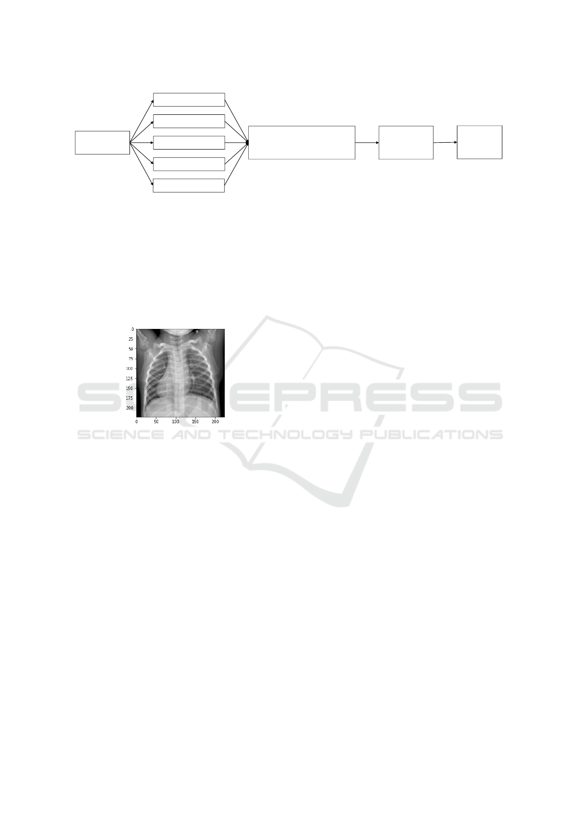
Input Image

224 x 224 x 3

DenseNet201

Xception

InceptionResNetV2

ResNet152V2

MobileNetV2

Linear combination of

Optimized Weights

with tuned hyper-parameters

Dense Layer

with Softmax

Activation

Output:

Normal/

Pneumonia

Figure 11: Weighted Average Ensemble.

ing time. Deep learning models are in general data-

hungry. They require a massive amount of data during

training to capture the most relevant features; other-

wise, the model does not generalize well when tested

on new data. Data Augmentation is a technique used

when the training data is limited to increase the train-

ing data size. This study augmented the training data

by randomly ﬂipping each image in a batch (see Fig-

ure 12).

Figure 12: Chest X-ray image ﬂipped left to right.

3.7 Hyper-parameter Tuning

Hyper-parameter tuning is one of the main contribu-

tions of this study. In the following subsections, we

brieﬂy discuss the parameters that are ﬁne-tuned dur-

ing training the model.

3.7.1 Learning Rate

The learning rate is one of the single most crucial

hyper-parameters to be carefully chosen while train-

ing the model. In other words, it would be equally

important to choose the appropriate learning rate for

the model to select the right model from a family of

models or learning algorithms. The typical values of

the learning rate while training a model with standard-

ized inputs, i.e., the inputs are in the interval (0, 1), are

greater than 1e-06 and less than 1 (Bengio, 2012).

Since we are using transfer learning with pre-

trained weights in this study, it is critical to have a

very low learning rate to avoid the risk of overﬁt-

ting very quickly. High learning rates apply larger

weight updates to the model. Therefore, it’s best to

avoid high learning rates as pre-trained models al-

ready hold decent weights that do not need larger

weight updates again while using them as transfer

learning models to train new datasets. Other common

strategies include learning rate warm-ups (He et al.,

2016a), (Goyal et al., 2017) and reducing the learn-

ing rate on the plateau, which is a part of callbacks

API in Keras (Cal, ). Learning rate warm-ups use less

aggressive learning rates at the start of training. The

other reduces the learning rate after a certain number

of epochs if the model does not improve the moni-

tored metrics, such as loss, accuracy, etc. during train-

ing.

In this study, the model’s training started with a

learning rate of 0.001 and then reduced the learning

rate by a factor of 0.3 for every ﬁve epochs if the

model did not improve. This strategy worked bet-

ter than others for the model to converge, where the

last reported learning rate was 2.7e-05, which helped

achieve the best model performance metrics.

3.7.2 Batch Size

Batch size is a conﬁgurable hyper-parameter during

the training of a neural network model, which refers

to the number of training examples used in a single

iteration. Generally, the batch size is between 10 and

1000, and 32 is a good default value according to

Bengio (Bengio, 2012). The Tensor Processing Unit

(TPU) was used to train the model, which consists of

four processors, and each of them has two TPU cores,

allowing eight cores for each TPU. We set a batch size

of 16 for each core of a TPU, with eight cores; the ﬁ-

nal batch size was 128.

3.7.3 Number of Epochs

The number of epochs or the number of training it-

erations is another hyper-parameter that can be op-

timized using the principle of Early stopping (Ben-

gio, 2012). Early stopping is another way of ensur-

ing that the model does not overﬁt the training data

by stopping the training process (see Figure 13), even

though other hyper-parameters such as learning rate

An Ensemble-based Approach by Fine-Tuning the Deep Transfer Learning Models to Classify Pneumonia from Chest X-Ray Images

397

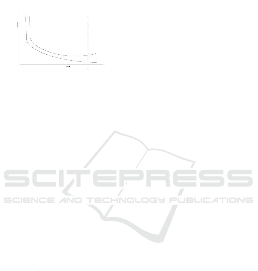
Epochs

Training

Validation

Early Stopping Epoch

Figure 13: Early Stopping.

and batch size would yield over-ﬁtting. Early stop-

ping comes as a callbacks API in Keras (Cal, ). The

patience parameter and the quantity to be monitored

are set to 20 and the loss. When the model shows no

improvement in the loss for 20 consecutive epochs,

the compiler terminates the training process.

3.8 Loss Function

The dataset has two classes (Normal, Pneumonia),

which is generally considered a binary classiﬁcation

problem(Normal - 0, Pneumonia - 1). In a binary clas-

siﬁcation task, we optimize the binary cross-entropy

function, so the model spits out whether the chest X-

ray image is Normal (0) or Pneumonia (1). In this

study, we modeled the algorithm to spit out the prob-

ability of the image being Normal or Pneumonia. So,

we intend to optimize the categorical cross-entropy

function instead of the binary cross-entropy function.

The categorical cross-entropy loss, also known as

log loss or logistic loss or softmax loss, is given by the

equation 5, where M is the number of training exam-

ples, K is the number of classes, y

is the target label

for training example m for class k, x is the input for

training example m, and h

is the model with neural

network weights θ.

cce

= −

∑

k=1

∑

m=1

× log (h

, k)) (5)

The predicted class probabilities are compared

with the actual classes/ labels (Normal, Pneumonia)

to minimize the loss. The loss is calculated that penal-

izes for any deviation between the actual class and the

model’s output. The penalty is a logarithmic loss that

yields larger scores for larger deviations, which tends

to 1, and smaller scores for small deviations tend to 0.

A perfect model will have a categorical cross-entropy

loss of 0.

3.9 Optimization Algorithm

After all the data preprocessing and hyper-parameters

conﬁguration, the next challenging task is choosing

the right optimization algorithm from a pool of opti-

mization algorithms, consisting of Gradient Descent

(GD), Stochastic Gradient Descent (SGD), Adam,

etc. Gradient Descent is the oldest and the traditional

optimization algorithm that solves the optimal value

along the gradient descent, converging at a linear rate.

In this method, the gradients of all the samples are

calculated for each parameter update making the gra-

dient descent cost calculation very high (Sun et al.,

2019). To overcome this issue, Robbins and Monro

(Robbins and Monro, 1951) proposed the Stochastic

Gradient Descent (SGD) optimization method. In this

method, the parameter updates are calculated using a

random sample from a mini-batch that converge at a

sub-linear rate. Even though the cost calculation is

improved, choosing an appropriate learning rate is of-

ten challenging. Kingma and Ba (Kingma and Ba,

2014) introduced Adam (Adaptive Moment Estima-

tion), a stochastic optimization algorithm based only

on ﬁrst-order gradients. The algorithm improves the

cost calculation with little memory and calculates in-

dividual adaptive learning rates for different param-

eters from the estimates of gradients’ ﬁrst and sec-

ond moments. The gradient descent process of the

Adam optimization method is relatively stable com-

pared to gradient descent and stochastic gradient de-

scent methods and is most suitable for large datasets

or parameters (Kingma and Ba, 2014). So, we used

Adam as an optimization algorithm in this study.

4 RESULTS

4.1 Classiﬁcation Performance Metrics

After ﬁnalizing the hyper-parameter conﬁgurations

and optimization algorithm, the models are compiled

and ﬁne-tuned during the training. The models’ per-

formance is evaluated on the test dataset, which con-

sists of 1,172 chest X-ray images, and the confu-

sion matrix is computed for each transfer learning

model consisting of True Negatives, False Positives,

False Negatives, and True Positives as shown in Ta-

ble 1. The Xception architecture performance is bet-

ter than all other transfer learning architectures, while

the weighted average ensemble outperformed every

transfer learning model, including the Xception archi-

tecture.

As mentioned in Section 3.3, the accuracy, pre-

cision, recall, and f1 score are calculated for each

ICAART 2021 - 13th International Conference on Agents and Artiﬁcial Intelligence

398

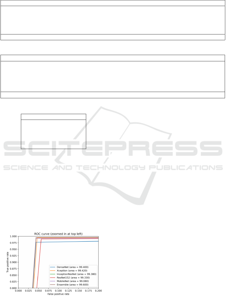
Table 1: Confusion Metrics.

Model True Negative (TN) False Positive (FP) False Negative (FN) True Positive (TP)

DenseNet201 303 14 7 848

Xception 302 15 5 850

InceptionResNet 303 14 7 848

ResNet152V2 299 18 9 846

MobileNetV2 303 14 7 848

Ensemble Model 303 14 4 851

Table 2: Classiﬁcation Performance Metrics.

Model Accuracy Precision Recall F1 Score AUC Test Loss Parameters

DenseNet201 98.21 98.38 99.18 98.78 99.40 0.09 18,096,770

Xception 98.30 98.27 99.42 98.84 99.42 0.11 20,811,050

InceptionResNet 98.21 98.38 99.18 98.78 99.38 0.09 54,279,266

ResNet152V2 97.7 97.92 98.95 98.43 99.33 0.11 58,192,002

MobileNetV2 98.21 98.38 99.18 98.78 99.08 0.11 2,226,434

Ensemble Model 98.46 98.38 99.53 98.96 99.60 0.08 162,638,991

Table 3: Weighted Average Ensemble Model Weights.

Model Weights

DenseNet201 0.22

Xception 0.29

InceptionResNet 0.18

ResNet152V2 0.17

MobileNetV2 0.15

transfer learning model (see Table 2). It is worth not-

ing that the results of MobileNetV2 architecture are

comparable to the best-performing architecture, i.e.,

the Xception architecture with approximately 20 mil-

lion trainable parameters, which is almost ten times

the MobileNet architecture. However, with about 162

million trainable parameters, the weighted average

ensemble model outperformed all other models with

test loss of 0.08 and achieving an accuracy of 98.46%,

precision of 98.38%, recall of 99.53%, f1 score of

98.96%, and AUC of 99.60% (See Figure 14). As

mentioned in Section 3.4, the weights are optimized

during training and the individual model weights are

Figure 14: Area under the Receiver Operating Characteris-

tics Curve (Zoomed in at the top left).

shown in Table3. The Xception and DenseNet201 ar-

chitectures account for more than 50% of the ﬁnal

predictions, with Xception architecture contributing

29% of the ﬁnal prediction and DenseNet201 archi-

tecture contributing 22% of the ﬁnal prediction.

4.2 Comparison of Results with Other

Recent Similar Works

In this section, we compare the results from our study

with other recent similar works (see Table 4, best per-

formance metrics are in bold). The results of our

weighted average ensemble model outperformed all

the classiﬁcation metrics such as accuracy, precision,

and f1 score, but recall and AUC from the comparable

works to accurate classiﬁcation of pneumonia.

5 CONCLUSION

According to the World Health Organization (WHO),

pneumonia is one of the world’s largest infectious

cause of death in children, particularly children under

the age of ﬁve (Pne, a) and Centers for Disease Con-

trol and Prevention (CDC) estimates that pneumonia

is one of the leading causes of death among adults

in the United States (Pne, b). Chest X-rays are the

standard technique used by radiologists in detecting

pneumonia, and even for the well-trained radiologist,

it is not uncommon to overlook pneumonia detection.

Due to the challenges of obtaining massive training

data mainly because of high annotation costs, we used

transfer learning techniques combined with data aug-

mentation to overcome overﬁtting during the model

An Ensemble-based Approach by Fine-Tuning the Deep Transfer Learning Models to Classify Pneumonia from Chest X-Ray Images

399

Table 4: Comparison of results with other recent similar works.

Accuracy Precision Recall F1 Score AUC

(Kermany et al., 2018) 92.80 87.20 93.20 90.10 96.80

(Rajaraman et al., 2018) 96.20 97.00 99.50 - 99.00

(Stephen et al., 2019) 93.73 - - - -

(Nahid et al., 2020) 97.92 98.38 97.47 97.97 -

(Chouhan et al., 2020) 96.39 93.28 99.62 96.35 99.34

(Hashmi et al., 2020) 98.43 98.26 99.00 98.63 99.76

(Mittal et al., 2020) 96.36 - - - -

(Rahman et al., 2020) 98.00 97.00 99.00 98.10 98.00

Current Work 98.46 98.38 99.53 98.96 99.60

training process. This study proposes a weighted av-

erage ensemble model by ﬁne-tuning the deep trans-

fer learning architectures to improve the classiﬁca-

tion performance metrics such as accuracy, precision,

recall, and f1 score to detect pneumonia from chest

X-ray images. To the best of our knowledge, we

achieved the best classiﬁcation performance metrics

ever reported in the literature for pneumonia classiﬁ-

cation with accuracy of 98.46%, precision of 98.38%,

and f1 score of 98.96%. Future work can include in-

vestigating the proposed ensemble model’s general-

ization ability in diagnosing other common diseases.

REFERENCES

Callbacks api. https://keras.io/api/callbacks/. (Accessed on

11/23/2020).

Cvpr2017. https://cvpr2017.thecvf.com/program/

main conference#cvpr2017 awards. (Accessed

on 10/31/2020).

Pneumonia. https://www.who.int/health-topics/pneumonia.

(Accessed on 10/26/2020).

Pneumonia — disease or condition of the week —

cdc. https://www.cdc.gov/dotw/pneumonia/index.

html. (Accessed on 10/26/2020).

Pneumonia: Symptoms, causes, diagnosis, treatment,

and complications. https://www.webmd.com/lung/

understanding-pneumonia-basics. (Accessed on

10/27/2020).

Use tpus — tensorﬂow core. https://www.tensorﬂow.org/

guide/tpu#input datasets. (Accessed on 11/04/2020).

Ayan, E. and

Unver, H. M. (2019). Diagnosis of pneu-

monia from chest x-ray images using deep learning.

In 2019 Scientiﬁc Meeting on Electrical-Electronics

& Biomedical Engineering and Computer Science

(EBBT), pages 1–5. IEEE.

Bengio, Y. (2012). Practical recommendations for gradient-

based training of deep architectures. In Neural net-

works: Tricks of the trade, pages 437–478. Springer.

Brown, G., Wyatt, J., Harris, R., and Yao, X. (2005). Di-

versity creation methods: a survey and categorisation.

Information Fusion, 6(1):5–20.

Chollet, F. (2017). Xception: Deep learning with depthwise

separable convolutions. In Proceedings of the IEEE

conference on computer vision and pattern recogni-

tion, pages 1251–1258.

Chouhan, V., Singh, S. K., Khamparia, A., Gupta, D., Ti-

wari, P., Moreira, C., Dama

sevi

cius, R., and De Albu-

querque, V. H. C. (2020). A novel transfer learning

based approach for pneumonia detection in chest x-

ray images. Applied Sciences, 10(2):559.

Dietterich, T. G. (2000). Ensemble methods in machine

learning. In International workshop on multiple clas-

siﬁer systems, pages 1–15. Springer.

Goyal, P., Doll

ar, P., Girshick, R., Noordhuis, P.,

Wesolowski, L., Kyrola, A., Tulloch, A., Jia, Y.,

and He, K. (2017). Accurate, large minibatch

sgd: Training imagenet in 1 hour. arXiv preprint

arXiv:1706.02677.

Hashmi, M. F., Katiyar, S., Keskar, A. G., Bokde, N. D.,

and Geem, Z. W. (2020). Efﬁcient pneumonia detec-

tion in chest xray images using deep transfer learning.

Diagnostics, 10(6):417.

He, K., Zhang, X., Ren, S., and Sun, J. (2016a). Deep resid-

ual learning for image recognition. In Proceedings of

the IEEE conference on computer vision and pattern

recognition, pages 770–778.

He, K., Zhang, X., Ren, S., and Sun, J. (2016b). Iden-

tity mappings in deep residual networks. In Euro-

pean conference on computer vision, pages 630–645.

Springer.

Huang, G., Liu, Z., Van Der Maaten, L., and Weinberger,

K. Q. (2017). Densely connected convolutional net-

works. In Proceedings of the IEEE conference on

computer vision and pattern recognition, pages 4700–

4708.

Kermany, D. S., Goldbaum, M., Cai, W., Valentim, C. C.,

Liang, H., Baxter, S. L., McKeown, A., Yang, G.,

Wu, X., Yan, F., et al. (2018). Identifying medical

diagnoses and treatable diseases by image-based deep

learning. Cell, 172(5):1122–1131.

Kingma, D. P. and Ba, J. (2014). Adam: A

method for stochastic optimization. arXiv preprint

arXiv:1412.6980.

Krizhevsky, A., Sutskever, I., and Hinton, G. E. (2012). Im-

agenet classiﬁcation with deep convolutional neural

networks. In Advances in neural information process-

ing systems, pages 1097–1105.

LeCun, Y., Bengio, Y., and Hinton, G. (2015). Deep learn-

ing. nature, 521(7553):436–444.

Liang, G. and Zheng, L. (2020). A transfer learning

ICAART 2021 - 13th International Conference on Agents and Artiﬁcial Intelligence

400

method with deep residual network for pediatric pneu-

monia diagnosis. Computer methods and programs in

biomedicine, 187:104964.

Litjens, G., Kooi, T., Bejnordi, B. E., Setio, A. A. A.,

Ciompi, F., Ghafoorian, M., Van Der Laak, J. A.,

Van Ginneken, B., and S

anchez, C. I. (2017). A survey

on deep learning in medical image analysis. Medical

image analysis, 42:60–88.

Lundervold, A. S. and Lundervold, A. (2019). An overview

of deep learning in medical imaging focusing on mri.

Zeitschrift f

ur Medizinische Physik, 29(2):102–127.

Mandell, L. A., Wunderink, R. G., Anzueto, A., Bartlett,

J. G., Campbell, G. D., Dean, N. C., Dowell, S. F.,

File Jr, T. M., Musher, D. M., Niederman, M. S.,

et al. (2007). Infectious diseases society of amer-

ica/american thoracic society consensus guidelines on

the management of community-acquired pneumonia

in adults. Clinical infectious diseases, 44(Supple-

ment

2):S27–S72.

Mittal, A., Kumar, D., Mittal, M., Saba, T., Abunadi, I.,

Rehman, A., and Roy, S. (2020). Detecting pneumo-

nia using convolutions and dynamic capsule routing

for chest x-ray images. Sensors, 20(4):1068.

Nahid, A.-A., Sikder, N., Bairagi, A. K., Razzaque, M., Ma-

sud, M., Z Kouzani, A., Mahmud, M., et al. (2020). A

novel method to identify pneumonia through analyz-

ing chest radiographs employing a multichannel con-

volutional neural network. Sensors, 20(12):3482.

Pan, S. J. and Yang, Q. (2009). A survey on transfer learn-

ing. IEEE Transactions on knowledge and data engi-

neering, 22(10):1345–1359.

Rahman, T., Chowdhury, M. E., Khandakar, A., Islam,

K. R., Islam, K. F., Mahbub, Z. B., Kadir, M. A., and

Kashem, S. (2020). Transfer learning with deep con-

volutional neural network (cnn) for pneumonia detec-

tion using chest x-ray. Applied Sciences, 10(9):3233.

Rajaraman, S., Candemir, S., Kim, I., Thoma, G., and An-

tani, S. (2018). Visualization and interpretation of

convolutional neural network predictions in detecting

pneumonia in pediatric chest radiographs. Applied

Sciences, 8(10):1715.

Robbins, H. and Monro, S. (1951). A stochastic approxi-

mation method. The annals of mathematical statistics,

pages 400–407.

Russakovsky, O., Deng, J., Su, H., Krause, J., Satheesh, S.,

Ma, S., Huang, Z., Karpathy, A., Khosla, A., Bern-

stein, M., et al. (2015). Imagenet large scale visual

recognition challenge. International journal of com-

puter vision, 115(3):211–252.

Sandler, M., Howard, A., Zhu, M., Zhmoginov, A., and

Chen, L.-C. (2018). Mobilenetv2: Inverted residu-

als and linear bottlenecks. In Proceedings of the IEEE

conference on computer vision and pattern recogni-

tion, pages 4510–4520.

Shahhosseini, M., Hu, G., and Pham, H. (2019). Opti-

mizing ensemble weights and hyperparameters of ma-

chine learning models for regression problems. arXiv

preprint arXiv:1908.05287.

Shen, D., Wu, G., and Suk, H.-I. (2017). Deep learning in

medical image analysis. Annual review of biomedical

engineering, 19:221–248.

Stephen, O., Sain, M., Maduh, U. J., and Jeong, D.-U.

(2019). An efﬁcient deep learning approach to pneu-

monia classiﬁcation in healthcare. Journal of health-

care engineering, 2019.

Sun, S., Cao, Z., Zhu, H., and Zhao, J. (2019). A survey

of optimization methods from a machine learning per-

spective. IEEE transactions on cybernetics.

Szegedy, C., Ioffe, S., Vanhoucke, V., and Alemi, A.

(2016a). Inception-v4, inception-resnet and the im-

pact of residual connections on learning. arXiv

preprint arXiv:1602.07261.

Szegedy, C., Vanhoucke, V., Ioffe, S., Shlens, J., and Wo-

jna, Z. (2016b). Rethinking the inception architecture

for computer vision. In Proceedings of the IEEE con-

ference on computer vision and pattern recognition,

pages 2818–2826.

Tan, C., Sun, F., Kong, T., Zhang, W., Yang, C., and Liu,

C. (2018). A survey on deep transfer learning. In

International conference on artiﬁcial neural networks,

pages 270–279. Springer.

Torrey, L. and Shavlik, J. (2010). Transfer learning. In

Handbook of research on machine learning appli-

cations and trends: algorithms, methods, and tech-

niques, pages 242–264. IGI global.

Weiss, K., Khoshgoftaar, T. M., and Wang, D. (2016).

A survey of transfer learning. Journal of Big data,

3(1):9.

An Ensemble-based Approach by Fine-Tuning the Deep Transfer Learning Models to Classify Pneumonia from Chest X-Ray Images

401