Flexibility in Home Delivery by Enabling Time Window Changes

F. Phillipson

and E. A. van Kempen

TNO, PO Box 96800, 2509 JE, The Hague, The Netherlands

Keywords:

Home Delivery, Vehicle Routing with Time Windows, Time Window Intervention, Incident Handling.

Abstract:

To enhance the perceived quality of home delivery services more and more ﬂexibility is offered to the re-

ceivers. Enabling same-day delivery, communicating predeﬁned narrow time windows, choosing the time

windows and alternative address delivery add to the receiver’s experience, making the delivery company an

interesting partner for parcel-shipping companies. A new ﬂexibility is the possibility to change the chosen

or communicated time window by the receiver during the day of delivery. In this paper we investigate the

effect on delivery costs of this ﬂexibility. Receivers are allowed to change their time window until the start of

the old or new (the earliest) time window. In this paper two situations are investigated: one situation where

communicated time window is a result of the planning process (Time Indication) and one situation where the

original time window was already chosen by the receiver (Time choice). We show that the costs rises quickly

in the Time Indication case when the percentage of time window changes grow. The Time Choice case is more

costly at the start, but time window changes can be handled without (too much) extra costs. However, here a

higher percentage of parcels is delivered outside the time windows.

1 INTRODUCTION

Last-mile delivery has become increasingly important

with the rise of e-commerce (Joerss et al., 2016). In

this last-mile delivery, the carrier transports the goods

sent by the shipper to the receiver. Here the ship-

per is the carrier’s customer and the receiver is the

shipper’s customer. To avoid ambiguities, we use

the terms carrier, shipper and receiver. The prob-

lems regarding an optimal last-mile delivery fall in

the area of Vehicle Routing Problems (VRP). Solving

the VRP might result in minimal costs for the carrier

or the shipper, but does not guarantee the (perceived)

quality of the shipment. Also, several issues arise

from home delivery activities for fulﬁlling those in-

ternet shopping orders, e.g., increased operating costs

for handing failed home deliveries, and deteriorated

trafﬁc conditions due to frequent delivery trips (Song

et al., 2016). An important factor for the (perceived)

quality of the delivery service is the variety of deliv-

ery options a receiver can choose from (Yao et al.,

2019; Rincon-Garcia et al., 2018; Gawor and Hoberg,

2019). Examples of delivery options are next-day de-

livery, same-day delivery, alternative address delivery

or predeﬁned time window delivery. Here, time win-

dows offer the beneﬁt of potentially serving as a com-

https://orcid.org/0000-0003-4580-7521

munication tool towards the receiver, allowing com-

panies to increase the success rate of their deliver-

ies. Naturally, a decrease in the number of delivery

failures will increase the receiver’s satisfaction level.

Nonetheless, as the implementation of time windows

reduces the efﬁciency of the routing, a trade-off has

to be made between receiver’s satisfaction and deliv-

ery costs (K

ohler et al., 2020). The possibilities to

improve the efﬁciency of home delivery are investi-

gated by (Van Duin et al., 2016). They conclude that

contact with the receiver can signiﬁcantly increase the

efﬁciency. In addition, a process called address intel-

ligence seems to hold great potential by using histori-

cal data as a way of predicting future deliveries. Other

promising options that apply to home delivery are the

possibility to use sliding time windows (Shao et al.,

2019) or to deliver at a different location, within a

predeﬁned time window or change the delivery time.

There is much work done on selection of time win-

dows sizes, e.g., (K

ohler et al., 2020; C

e et al.,

2019; Mackert, 2019; Klein et al., 2019; Hernandez

et al., 2017). The work of (Agatz et al., 2011) tackles

the problem of selecting time windows to offer in dif-

ferent regions. In other words, receivers in certain re-

gions are provided with speciﬁc choices to accommo-

date the ability to construct cost efﬁcient routes. The

results emphasise the trade-off between delivery efﬁ-

Phillipson, F. and van Kempen, E.

Flexibility in Home Delivery by Enabling Time Window Changes.

DOI: 10.5220/0010330604530458

In Proceedings of the 10th International Conference on Operations Research and Enterprise Systems (ICORES 2021), pages 453-458

ISBN: 978-989-758-485-5

453

ciency and receiver’s satisfaction since offering nar-

row time windows is convenient for the receiver but

greatly reduces the efﬁciency of the routes.

To improve the perceived quality and receiver’s satis-

faction even more, more ﬂexibility can be offered to

the receivers, for example the possibility to change the

delivery time window or place during the day of deliv-

ery. Again this reduces the efﬁciency of the routing.

In this paper we study the effect of offering the ﬂex-

ibility to change the time window of delivery during

the day of delivery and give insight in the cost of this

ﬂexibility in terms of driving time and vehicle kilo-

metres. Where there are papers on incident handling

and disruption management, we will however simply

execute re-planning before every new time window.

A general overview of papers that look at disruption

management in VRPs can be found in (Eglese and

Zambirinis, 2018). Yang et al. (Yang et al., 2017)

provide a incident handling method in case of time

window changes. We want to allow these changes and

are interested in the effect these changes have on the

operational costs. We are not aware of other papers

that are doing this and this option is not taken into ac-

count in large literature overviews like (Boysen et al.,

2020) and (Savelsbergh and Van Woensel, 2016).

In this paper we investigate the effect of offering

the ﬂexibility to change the delivery time window by

the receiver. In Section 2 we start with the descrip-

tion of the case we consider, explain the assumptions

we make and elaborate on the simulation approach we

use. The results of this simulation approach are pre-

sented in Section 3. Finally, in Section 4 we discuss

the results, draw some conclusions and suggest topics

for further research.

2 ASSUMPTIONS AND

APPROACH

We consider a regional depot from which parcels are

distributed over a certain area. Parcels arrive at night

and are assigned to vehicles. This problem can be

modelled as a VRP. We assume that this VRP was

solved for this certain depot and that, at the begin-

ning of the morning, the vehicles are loaded for their

route. Next, receivers are informed about a delivery

time window or time slot. For the way this is organ-

ised, we consider two cases:

• The VRP is solved and thus the routes of the ve-

hicles are optimised without giving the receivers

the possibility to choose a time slot. The indica-

tion the receiver obtain is a result of the optimisa-

tion. We will call this Time Indication. The VRP

is an NP-hard problem (Lenstra and Rinnooy Kan,

1981).

• The VRP is solved with time windows (VRPTW)

and thus the routes of the vehicles are optimised

based on the preference of the receivers. The in-

dication the receivers obtain is a result of the opti-

misation under the constraint of these preferences.

We will call this Time Choice. The VRP-TW is

also an NP-hard problem (Dror, 1994).

Both cases will be considered using two different time

window lengths: 1 hour (not overlapping) and 3 hours

(1 hour overlapping). So the ﬁrst category consists of

the time windows 9-10, 10-11, etc., the second cate-

gory consists of the time windows 9-12, 11-14, 13-16

etc.

We now introduce the possibility for the receivers

to change their time windows. The only restric-

tion they have, is that they have to communicate this

change before the start of their current time window

and before the start of their newly chosen time win-

dow. This means, in the case of the 3-hour time win-

dows, that when the receiver got assigned the time

window 11-14h and he wants to change this to 13-

16h, this has to be communicated before 11h. In the

case that the receiver got assigned the time window

15-18h and he wants to change this to 13-16h, this

has to be communicated before 13h.

We will restrict the case to a single vehicle. This

vehicle delivers the parcels to the receivers. The size

of the areas we consider is based on real data and the

number of parcels that is considered is based on the

number of parcels that can be delivered in that area

within a working day of (around) eight hours. This

assumption resulted in two areas, one with a size of

6 km

and 120 parcels to deliver, the other area has

a size of 54 km

km and 90 parcels to deliver. We

use real (ﬁxed) deliver areas from practice, however,

within this are we generate address data randomly for

50 days and a delivery time window for each address.

Now we calculate for each day the optimal route in

two ways:

1. The optimal route without time windows.

2. The (approximate) optimal route with time win-

dows.

The ﬁrst route is used as benchmark. From this ﬁrst

route the Time Indication case is derived. The result-

ing times from this optimal route are communicated

to the receivers. From the huge number of optimisa-

tion techniques, as shown in (Psaraftis et al., 2016),

for the second route we have chosen to use a simu-

lated annealing approach (using the implementation

of yarpiz.com). The parameters, the number of it-

erations, the initial temperature and the temperature

ICORES 2021 - 10th International Conference on Operations Research and Enterprise Systems

454

damping rate, are chosen such that (without the time

window constraints) it gives the same results as the

ﬁrst route. With this parameters the route with time

window constraints, the Time Choice case, is calcu-

lated and communicated (conﬁrmed) to the receivers.

Now for each day, the course of the day is simu-

lated. Over all the receivers a percentage p is selected

that is assigned a new delivery window. Of course,

this assignment simulates the ﬂexibility the receiver

has in real life to change the delivery window him-

self. We assume this information gets available at the

latest moment possible, compliant to the restriction

the receiver has in changing the delivery time. During

the simulation, at the start of each delivery window,

a new (approximate) optimal plan is recalculated, us-

ing the latest delivery window information. This plan

is executed until the beginning of the next delivery

window. Note that a continuous updating scheme, or

at least updating at each moment new information is

revealed, and the availability of this information ear-

lier that the latest moment possible, will increase the

performance of this approach. This means that the

extra costs of introducing this ﬂexibility is lower than

presented in this paper, which can be considered as a

worst case.

3 RESULTS

As indicated, we did this simulation for the two ar-

eas, for the two time slot lengths, for ﬁve percentages

(p = 5%, 15%, 25%, 35% and 45%) and for the cases

Time-Indication and Time-Choice. Each simulation

was repeated 50 times to get a (statistically) reliable

answer.

In Figures 1-3 the results are presented for the 6

area. We present the results relative to the gen-

eral Time Indication solution. In the actual results,

approximately 50 kilometre is already taken by going

to and from the depot. In analysing the relative dif-

ferences we will exclude this 50 kilometres. Then,

as expected, the optimal route with Time Indication

is the route with the lowest travel distance. If we in-

troduce time interventions (both with 1h and 3h time

windows) to this route, from 5 to 45% of the receivers,

we see an increase in distance travelled in Figure 1.

The more receivers ask for a change in delivery win-

dow, the higher the costs in kilometres, going up by

86% (from 30 to 55 kilometres, subtracting the 50

kilometres) in the case of the 1 hour time window

and by 122% in case of the 3 hour time window at

the point of 45% of the receivers realising time inter-

ventions. Note that the two time windows start at the

same value, caused by the fact that there is no dif-

ference in starting solution. The only difference is

the length of the delivery window they get communi-

cated. However, in the case of time interventions the

costs in kilometres rises more quickly for the 1-hour

case.

Then we go to the result of the case Time Choice

without time interventions. Receivers can choose

their own delivery window from the start. Now, see

Figure 2 the travel distance already goes up by 113%

for the 3 hour case and even with 225% for the 1

hour case. In fact, instead of one tour in the deliv-

ery area, the vehicles drives a number of tours equal

to the number of time-windows. Introducing the pos-

sibility to change the time window here hardly has

an effect, as can be seen in Figure 3. In the 3 hour

time window case there is enough slack and possibil-

ities to change the routes without effecting the num-

ber of kilometres driven. In the 1 hour time windows

it comes with a small cost. However, in both cases

the number of kilometres is independent of the per-

centage of changes. The solution is already disturbed

enough that it can handle any number of change. The

(small) rise of costs is caused by the less efﬁcient rout-

ing from and to the depot.

In ﬁgure 4 all the results are presented for the 54

area. We see largely the same results, where

the gaps between the cases with and without time-

interventions for the Time Choice cases are a bit

larger, due to the larger distances. We also see that

the 1h and 3h time windows for the Time Indication

have almost the same course.

The results for the Time Indication case with time

interventions are equal. However, what is not de-

picted in the costs is the number of deliveries outside

the communicated time windows. For the Time Indi-

cation case with the 3 hour (overlapping) time win-

dows, all the receivers can be delivered within their

time windows for all percentages of time interven-

tions. For the 1 hour time window this is not the case.

On average 4% up to 8% of the deliveries are outside

the time window. For the Time Choice case this is

much worse. Here introducing the time interventions

for the 3 hour time windows give 26% late deliveries

and in the 1 hour time windows case even 40-60%.

This means that introducing time interventions in a

big(ger) area with tight time windows might not incur

(that much) extra distance, it dramatically deteriorates

the quality of the delivery service.

Flexibility in Home Delivery by Enabling Time Window Changes

455

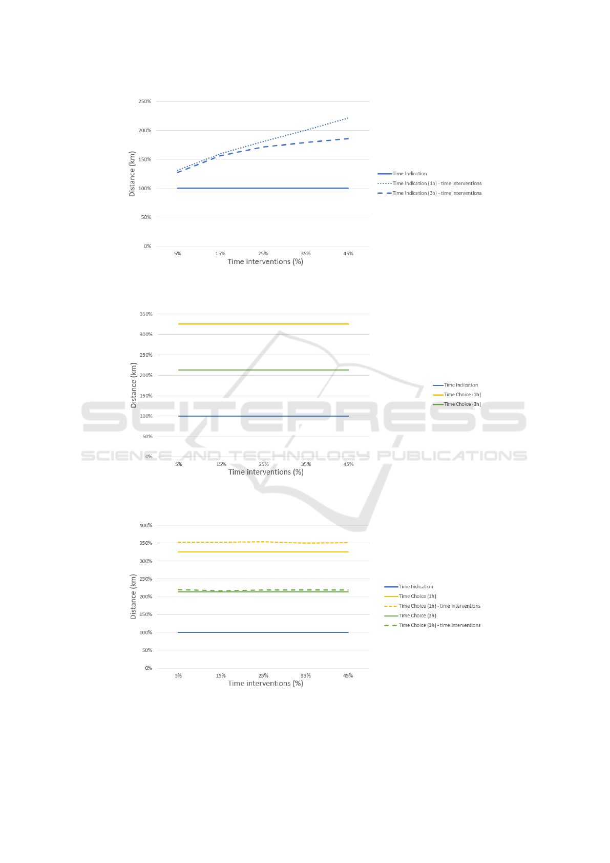
Figure 1: Result of introducing time interventions to the Time Indication case. The distance is given relative to the general

Time Indication case. A 1 hour time indication with time interventions leads to the highest costs and costs rise more quickly

if more interventions are made.

Figure 2: Result of giving receivers the possibility to choose a 1-hour or 3-hour delivery window. The distance is given relative

to the general Time Indication case. Choice for a 1-hour time window increases costs by 225% compared to a scenario where

receivers are given a time indication.

Figure 3: Result of introducing time interventions to the Time Choice case. The distance is given relative to the general Time

Indication case. Introducing the possibility to change a chosen time-window has a marginal effect on the costs for both the 1

hour and 3 hour time windows.

ICORES 2021 - 10th International Conference on Operations Research and Enterprise Systems

456

Figure 4: Results for the 54 km

area. Largely the same results as earlier. Note that the gaps for the Time Choise cases are

bigger.

4 DISCUSSION AND

CONCLUSIONS

In the previous section we saw how much the travel

distance increases when enabling the end-customers

to change the communicated or chosen time windows.

In the case of Time Indication, where the end-users

cannot choose their initial time window but are only

informed about their time window, this increase is de-

pendent on the percentage of receivers that uses this

possibility. In the case of Time Choice, where the re-

ceivers have chosen the time window, which already

provides an increase of travel distance, the system is

robust enough to absorb these disturbances.

Note that we started with the assumption ‘the

number of parcels that is considered is based on the

number of parcels that can be delivered in that area

within a working day of (around) eight hours’. That

means that all solution other than the Time Indica-

tion starting point without time interventions will take

more than eight hours and will not be feasible within

one shift. For the small area, the 6 km

area, the

Time Choice base case with 3 hour time windows

takes around 11 hours, the 1 hour time windows case

with time interventions takes even around 16 hours.

This means that these routes actually will cost much

more that the distances shown in Figures 1-4. It will

come with the costs of an extra driver, an extra vehicle

and extra kilometres from the depot to the distribution

area for this vehicle.

What we also see is how much ﬂexibility can be

offered in the Time Indication case before it is (al-

most) as costly to introduce Time Choice as an alter-

native, apart from the implementation costs of a Time

Choice system. Most carriers do not have direct con-

tact with the receivers, so this has to be organised to-

gether with their customers, the shippers.

As possibility for further research we see the fol-

lowing topics. First, we could validate in practice

what the preferences of receivers are. This impacts

the strategic decisions to be made by the carrier. Sec-

ond, as said earlier, we could take into account the

total costs of the time-interventions by only accepting

plans (after time-interventions) that can be executed

within the limitations of working hours.

ACKNOWLEDGEMENTS

The authors like to thank the Dutch Topsector Lo-

gistics (TKI Dinalog and NWO) for the support to

Project SOLiD (NWO project number 439.17.551).

The aims of the SoliD project (Quak et al., 2019) is

to bridge the gap between the long(er) term vision

and the short term daily logistics operations in self-

organising parcel distribution. It provides an impulse

for self-organising logistics as well as a more concrete

perspective / way of thinking for logistics practition-

ers with respect to opportunities for new logistics ser-

vices or activities that on the short term can be ex-

pected by taking the mentioned developments in ac-

count.

REFERENCES

Agatz, N., Campbell, A., Fleischmann, M., and Savels-

bergh, M. (2011). Time slot management in attended

home delivery. Transportation Science, 45(3):435–

449.

Flexibility in Home Delivery by Enabling Time Window Changes

457

Boysen, N., Fedtke, S., and Schwerdfeger, S. (2020). Last-

mile delivery concepts: a survey from an operational

research perspective. OR Spectrum, pages 1–58.

e, J.-F., Mansini, R., and Raffaele, A. (2019). Tactical

Time Window Management in Attended Home Deliv-

ery. CIRRELT, Centre interuniversitaire de recherche

sur les r

eseaux d’entreprise .

Dror, M. (1994). Note on the complexity of the shortest path

models for column generation in vrptw. Operations

Research, 42(5):977–978.

Eglese, R. and Zambirinis, S. (2018). Disruption manage-

ment in vehicle routing and scheduling for road freight

transport: a review. Top, 26(1):1–17.

Gawor, T. and Hoberg, K. (2019). Customers valuation of

time and convenience in e-fulﬁllment. International

Journal of Physical Distribution & Logistics Manage-

ment.

Hernandez, F., Gendreau, M., and Potvin, J.-Y. (2017).

Heuristics for tactical time slot management: a pe-

riodic vehicle routing problem view. International

transactions in operational research, 24(6):1233–

1252.

Joerss, M., Neuhaus, F., and Schr

oder, J. (2016). How

customer demands are reshaping lastmile delivery.

Travel, Transport & Logistics, 1:4.

Klein, R., Neugebauer, M., Ratkovitch, D., and Steinhardt,

C. (2019). Differentiated time slot pricing under rout-

ing considerations in attended home delivery. Trans-

portation Science, 53(1):236–255.

ohler, C., Ehmke, J. F., and Campbell, A. M. (2020). Flex-

ible time window management for attended home de-

liveries. Omega, 91:102023.

Lenstra, J. K. and Rinnooy Kan, A. H. G. (1981). Com-

plexity of vehicle routing and scheduling problems.

Networks, 11(2):221–227.

Mackert, J. (2019). Choice-based dynamic time slot man-

agement in attended home delivery. Computers & In-

dustrial Engineering, 129:333–345.

Psaraftis, H. N., Wen, M., and Kontovas, C. A. (2016). Dy-

namic vehicle routing problems: Three decades and

counting. Networks, 67(1):3–31.

Quak, H., van Kempen, E., van Dijk, B., and Phillipson, F.

(2019). Self-organization in parcel distribution-solid’s

ﬁrst results. In IPIC 2019 6th International Physical

Internet Conference London 2019.

Rincon-Garcia, N., Waterson, B., Cherrett, T. J., and

Salazar-Arrieta, F. (2018). A metaheuristic for the

time-dependent vehicle routing problem considering

driving hours regulations–an application in city lo-

gistics. Transportation Research Part A: Policy and

Practice.

Savelsbergh, M. and Van Woensel, T. (2016). 50th anniver-

sary invited articlecity logistics: Challenges and op-

portunities. Transportation Science, 50(2):579–590.

Shao, S., Xu, G., Li, M., and Huang, G. Q. (2019). Syn-

chronizing e-commerce city logistics with sliding time

windows. Transportation Research Part E: Logistics

and Transportation Review, 123:17–28.

Song, L., Wang, J., Liu, C., and Bian, Q. (2016). Quanti-

fying beneﬁts of alternative home delivery operations

on transport in china. In 2016 16th International Con-

ference on Control, Automation and Systems (ICCAS),

pages 810–815.

Van Duin, J., De Goffau, W., Wiegmans, B., Tavasszy, L.,

and Saes, M. (2016). Improving home delivery ef-

ﬁciency by using principles of address intelligence

for b2c deliveries. Transportation Research Procedia,

12:14–25.

Yang, H., Zhao, L., Ye, D., and Ma, J. (2017). Distur-

bance management for vehicle routing with time win-

dow changes. Operational Research, pages 1–20.

Yao, Y., Zhu, X., Dong, H., Wu, S., Wu, H., Tong, L. C.,

and Zhou, X. (2019). ADMM-based problem decom-

position scheme for vehicle routing problem with time

windows. Transportation Research Part B: Method-

ological, 129:156–174.

ICORES 2021 - 10th International Conference on Operations Research and Enterprise Systems

458