Planning with Hierarchical Temporal Memory for Deterministic Markov
Decision Problem
Petr Kuderov
1 a
and Aleksandr I. Panov
1,2 b
1
Moscow Institute of Physics and Technology, Moscow, Russia
2
Artificial Intelligence Research Institute, Federal Research Center “Computer Science and Control” of the Russian
Academy of Sciences, Moscow, Russia
Keywords:
Model-based Reinforcement Learning, Markov Decision Process, Planning, Hierarchical Temporal Memory,
Sparse Distributed Representation.
Abstract:
Sequential decision making is among the key problems in Artificial Intelligence. It can be formalized as
Markov Decision Process (MDP). One approach to solve it, called model-based Reinforcement Learning
(RL), combines learning the model of the environment and the global policy. Having a good model of the
environment opens up such properties as data efficiency and targeted exploration. While most of the memory-
based approaches are based on using Artificial Neural Networks (ANNs), in our work we instead draw the
ideas from Hierarchical Temporal Memory (HTM) framework, which is based on human-like memory model.
We utilize it to build an agent’s memory that learns the environment dynamics. We also accompany it with an
example of planning algorithm, that enables the agent to solve RL tasks.
1 INTRODUCTION
Reinforcement Learning (RL) seeks to find meth-
ods that enable robots or virtual agents to act au-
tonomously in order to solve human-defined tasks. It
requires from such methods to learn a policy for se-
quential decision-making problems, which are com-
monly formalized as MDP optimization (Puterman,
1994). Recently, RL has achieved notable landmarks
in various task domains such as classical board games
chess (Campbell et al., 2002), Go (Silver et al., 2016),
poker (Brown and Sandholm, 2017) and visually rich
computer games like Atari (Mnih et al., 2015) and
Dota 2 (Berner et al., 2019). At the core of some of
the methods used, especially for board games, were
planning algorithms, which rely on the knowledge of
the environment dynamics. However, the model of
the environment is unknown in general case, and there
are two common opposite approaches in RL to deal
with it: a model-free and a model-based.
Model-free approach doesn’t explicitly learn and
make use of the knowledge of the environment. In-
stead, it directly learns the global policy from inter-
actions with the environment. While model-free ap-
a
https://orcid.org/0000-0001-7055-3426
b
https://orcid.org/0000-0002-9747-3837
proach has many successful examples among its dis-
advantages are data inefficiency as it requires high
amount of interactions with the environment and
struggles for precise lookahead (Mnih et al., 2015;
Haarnoja et al., 2018; Schulman et al., 2017).
Model-based RL can address the issues of both
planning and model-free RL by first learning the envi-
ronment dynamics and then to exploit it for more ef-
ficient learning of the agent’s policy (Moerland et al.,
2020). Typically, the model is represented by MDP
and consists of two components: a state transition
model and a reward model. After the model has
been learned, MDP planning method, such as MCTS
(Coulom, 2007), can be applied to infer the optimal
policy. One model-based RL approach is to build
a model that operates on the raw input data level
(Gorodetskiy et al., 2020; Kaiser et al., 2020). For
visually rich environments this may be expensive in
terms of computations and also may lead to a model
attentive to unimportant details. Another approach is
to build a more compact latent-space model instead,
for example, to represent an abstract MDP equivalent
to the real one in terms of state values (Schrittwieser
et al., 2020).
To model the environment it’s common to use Ar-
tificial Neural Networks (ANNs) (Schrittwieser et al.,
2020; Ha and Schmidhuber, 2018). But it’s also very
Kuderov, P. and Panov, A.
Planning with Hierarchical Temporal Memory for Deterministic Markov Decision Problem.
DOI: 10.5220/0010317710731081
In Proceedings of the 13th International Conference on Agents and Artificial Intelligence (ICAART 2021) - Volume 2, pages 1073-1081
ISBN: 978-989-758-484-8
Copyright
c
 2021 by SCITEPRESS – Science and Technology Publications, Lda. All rights reserved
1073

Figure 1: Two examples of generated 5x5 maze environ-
ments. Walls - dark purple, starting agent’s position - yel-
low, rewarding goal state - salad.
tempting to take more inspiration from human brains,
especially for how our memory functions (Hassabis
et al., 2017). Hierarchical Temporal Memory (HTM)
framework (George and Hawkins, 2009) is an exam-
ple of such human-like memory model. This frame-
work utilizes discrete binary sparse distributed repre-
sentations (SDR) (Cui et al., 2017) that enables more
efficient data processing, high noise tolerance and a
natural way to set similarity metric between data em-
beddings. HTM also provides a model of the sequen-
tial temporal memory (TM) (Hawkins and Ahmad,
2016). Learning in TM isn’t based on the gradient
descend, and typically it learns with a faster rate com-
pared to common ANNs.
In our work we present a simplified memory-
based framework based on the ideas of HTM that
can be used to model the environment dynamics, sup-
plied with the planning algorithm to infer the opti-
mal global policy. Some attempts to extend the HTM
model have been made before (Skrynnik et al., 2016;
Daylidyonok et al., 2019; Nugamanov and Panov,
2020), but the full implementation of the planning
subsystem with consideration for reinforcement sig-
nal was not implemented in other works. We study
applicability of the presented memory model and vi-
ability of the planning method in different maze envi-
ronments.
2 BACKGROUND
2.1 Reinforcement Learning
In this paper we consider the classic decision-making
problem with an agent operating in an environ-
ment that is formalized as Markov Decision Process
(MDP). As a starting point in our research we sim-
plify the problem assuming that the environment is
fully observable and deterministic. We also consider
only environments with the distinctive goal-oriented
tasks, where an agent is expected to reach desirable
goal state in a limited time.
Therefore, MDP is defined as a tuple M =
(S , A , R, P, s
0
, s
g
), where S = {1, . . . , s
n
} is the state
space of the environment, A = {1, . . . , a
m
} is the ac-
tion space available to an agent, and s
0
and s
g
are the
initial and the goal state distributions respectively. At
each time step t, an agent observes a state s
t
∈ S and
selects an action a
t
∈ A . As a result, it receives the
reward r
t
∈ R(s
t
, a
t
) and transitions to the new state
s
t+1
= P(s
t
, a
t
). An agent’s policy π : S → A is a
mapping from a state to an action. The agent’s goal is
to maximize the expected return E [
∑
∞
t=0
r
t
].
We don’t use discount factor γ in the return calcu-
lation. Instead, we assume that the reward function is
designed the way that it highly rewards reaching the
goal states and slightly punishes reaching any other
states - it should reflect the goal-oriented nature of the
environments that were taken into consideration.
2.2 Temporal Memory
Temporal Memory (TM) from Hierarchical Temporal
Memory (HTM) framework is a model of the sequen-
tial memory. It works with sparse distributed repre-
sentations (SDR), i.e. sparse binary vectors, which
are typically high-dimensional. Therefore, the data
encoding scheme should be chosen too. In 3.1 we
describe how agent’s memory is organized on top of
TM, so this section mostly covers the TM’s input.
In our work both actions and states are represented
as integer numbers from a fixed range (although, dif-
ferent for states and actions). Thus, we use a simple
encoding scheme, where numbers from some range
[0, N) are mapped to non-overlapping equally-sized
sets of active bits of the output SDR vector. For ex-
ample for N = 3 numbers 0, 1 and 2 are encoded cor-
respondingly as following:
0 → 1111 0000 0000
1 → 0000 1111 0000
2 → 0000 0000 1111
As you see, resulting vector is split into buckets of
bits, and the size of buckets is a hyperparameter (in
the example above it’s 4).
For SDR vectors a union operation is defined as
a bitwise OR applied to the corresponding vectors.
Also we define a similarity metric, which is the num-
ber of the same one-bits of the vectors in considera-
tion, which is, again, the same as the dot product of
such vectors.
Temporal Memory model provides algorithms not
only to learn sequences of SDR vectors [v
0
, v
1
, v
2
, . . . ]
but also to make predictions about what SDR vector v
0
ICAART 2021 - 13th International Conference on Agents and Artificial Intelligence
1074

Figure 2: Schematic view of our agent and its training loop.
comes next based on the past experience. The predic-
tion is represented as an SDR vector too - it’s a union
of SDR vectors v
0
= ∪v
o
i
, where each vector v
o
i
rep-
resents a single separate expected outcome. Notice
that as the union of SDR vectors is also an SDR vec-
tor, TM model allows working simultaneously with
the unions of sequences as well.
3 PLANNING WITH TEMPORAL
MEMORY
In our method we train an agent to reach a reward-
ing goal state s
g
. Agent isn’t explicitly provided
with the goal it should reach, but it’s allowed to re-
member epxerienced rewarding states. An agent is
supplied with the memory module to learn the envi-
ronment’s dynamics and a planning algorithm which
heavily relies on the learned model (see Fig. 2).
The planning algorithm constructs a plan of actions
p = [a
t
, a
t+1
, . . . , a
t+h−1
] that leads to the desired state
s
g
= s
t+h
from the current state s
t
. In case if the
planning algorithm fails to provide a plan the agent
is switched to the exploration strategy π
r
in order
to improve the learned model. As the result at each
timestep an agent operates either according to a con-
structed plan p or according to the random uniformly-
distributed exploration policy π
r
.
3.1 Memory Module
The agent’s memory module consists of two sub-
modules. One submodule, called transition memory,
learns the transition model f : S × A → S of the
environment, while the other, called goal states mem-
ory, keeps track of the past rewarding goal states s
g
.
Consider a trajectory of an agent τ =
[s
0
, a
0
, r
0
, s
1
, a
1
, r
1
, . . . , r
T −1
, s
T
]. Each pair (s
t
, a
t
) at
the moment t defines the precondition to the transi-
tion in the environment (s
t
, a
t
) → s
t+1
. Therefore,
we made transition memory to learn the sequences of
such transitions Tr = [(s
0
, a
0
), (s
1
, a
1
), . . . ] from the
trajectories that the agent produces. The learning is
performed in an online fashion, i.e. at each timestep.
The transition memory submodule is based on a
Temporal Memory. To encode each state-action pair
(s, a) we use two separate integer encoders for states
and actions respectively to obtain binary sparse vec-
tors. The states encoder maps integer numbers from
[0, |S |) range, and the actions encoder maps integer
numbers from [0, |A |) range. As most of the time our
method works with SDR, for simplicity further on we
use the same notation s and a for state’s and action’s
corresponding SDR too. To work with pairs (s, a) we
just concatenate their respective SDR vectors together
into one. For any given state-action pair (s, a) the
transition memory submodule can give a prediction
on what state s
0
is coming next. Precisely, it allows
prediction queries of the form:
given a superposition of states S = ∪s
i
and a
superposition of actions A = ∪a
j
, what super-
position of next states S
0
= ∪s
0
m
all possible
state-action pairs (s
i
, a
j
) lead to?
Here by superpositions of states (or actions) we mean
a union of their respective SDR vectors. By calling it
not just a union we emphasize that the SDR vectors
defining a union are meaningful. Note also that once
a superposition SDR vector is obtained you cannot
simply split it back into the origins formed it
1
.
Under certain conditions the transition memory
submodule can also be used backward - as an inverse
of an environment transition function f . This feature
becomes available after getting the result to a predic-
tion query and only for the states s
0
m
that match the
result S
0
= ∪s
0
m
. For each such state s
0
it can provide
which state-action pairs from the original query lead
to s
0
: {(s, a)} = f
−1
(s
0
). Notice that in general case
it’s possible that a multiple state-action pairs lead to
s
0
.
1
However, encoding scheme used maps different states
or actions to non-overlapping sets of bits. That keeps them
easily distinguishable from each other even in a superposi-
tion. Non-overlapping scheme makes things simpler to read
and debug, but it has a crucial downside too - it cannot pre-
serve possible similarity between states (or observations).
So we made the planning algorithm only to require a sepa-
ration of the state bits from the action bits in a state-action
pair SDR (s, a), which means it respects that origin SDRs
cannot be induced from a superposition. In future works we
plan experimenting with more complex environments and
visually rich observations, therefore the transition to over-
lapping encoding scheme seems inevitable, hence it has al-
ready been reflected in the planning algorithm.
Planning with Hierarchical Temporal Memory for Deterministic Markov Decision Problem
1075

3.2 Planning Algorithm
The goal of planning is to find a plan of actions
p = [a
t
, a
t+1
, . . . , a
t+h−1
] that leads to the desired state
s
g
= s
t+h
from the current state s
t
. We restrict result-
ing plan to have no more than H actions. Therefore,
H defines a planning horizon of an agent.
Planning process is split into two stages. It starts
with the forward planning from the current state s
t
until a rewarding goal state s
g
is reached. At this
stage the planning algorithm operates with superposi-
tions and cannot track the exact path to the goal state.
Because of that it proceeds then to the backtracking
stage, during which the exact path from the reached
goal state back to the starting state s
t
is deduced.
3.2.1 Forward Planning
In our method an agent uses its experience and ex-
pects the reward to be in one of the rewarding goals
states from the previous episodes. But even if that’s
not true, we still expect that the direct goal-based ex-
ploration could be more optimal for an agent than
pure random walking. Hence we set the agent to keep
track of previous rewarding states using its goal track-
ing memory submodule. We give such goal states a
priority.
Consider that at some timestep t
0
an agent is in
state s
0
. To find out if there is a reachable goal state in
a radius of H actions, we start planning from the state-
action superposition (S
0
= s
0
, A = ∪a
i
)
2
, where A is
a superposition of all available actions (see Alg. 1).
One step of the planning is just the transition mem-
ory submodule making a prediction. This gives us a
superposition of the state-action pairs expected to go
next. Predicting for a superposition (S
0
= s
0
, A = ∪a
i
)
is similar to making all possible actions from the state
s
0
simultaneously in parallel and getting the result of
all possible outcomes entangled together into a single
superposition SDR vector. However, we still can split
the resulting superposition into the pair of states su-
perposition and actions superpositions, because it is
just a concatenation of independent parts.
After the first planning step we have a superpo-
sition of the next states S
1
= ∪s
i
1
, reachable in one
agent’s action. To get all reachable states in two
agent’s action, we repeat prediction step, now from
the superposition (S
1
, A). Again, it’s similar to mak-
ing all possible actions from each of the next states in
S
1
.
This prediction process continues until either one
of the tracked goal states is reached, or planning hori-
2
We use superscripts for action indices here to avoid
messing with subscripts denoting the timestep.
Algorithm 1: Forward Planning.
Data: s
0
- initial state
sa
0
← (s
0
, A) // starting superposition
Θ ← [] // active segments history
for i ← 0, . . . , H − 1 do
memory.ActivatePredict(sa
i
)
Θ[i] ← memory.active segments
(S
i
, A
i
) ← PredictionFromSegments(Θ[i])
sa
i+1
← (S
i
, A)
reached goal ← MatchGoals(S
i
)
if reached goal 6= /0 then
return reached goal, Θ
return /0
zon limit is exceeded. In the former case the planning
algorithm proceeds to the next stage. In the latter,
we cancel it, and an agent has to use random strat-
egy to make a move before it tries to plan again. To
test if any of the tracked goal states is reached at i-th
planning step, we calculate similarity between each of
their SDR vectors and i-th superposition S
i
. The goal
state is considered presented in S
i
superposition, and
therefore reached during the forward planning, if its
similirity is over some predefined threshold.
During this stage we also collect a history of active
superpositions Θ = [S
0
, S
1
, . . . S
h
]. In more details, we
keep the track of Temporal Memory cells’ segments
activations. Each segment is a pair (p, {c
i
}), where p
- an index of the predicted cell and {c
i
} is a set of cell
indices that induce prediction of p. This information
allows us to provide the transition memory submod-
ule with an inversed transition function f
−1
discussed
in Sec. 3.1. Thus, the transition memory submodule
can answer which {(s, a)} has lead to a state s
0
by
tracking which cells predicted s
0
cells.
It’s possible to find multiple reachable goals at the
end of this stage. In our current implementation we
use the first matched from the set of tracked goals.
3.2.2 Backtracking
After the first stage the planning algorithm “believes”
that some goal state g = s
h
can be reached in h
steps. The problem is that it doesn’t know how to
get there because until now it worked with superpo-
sitions. Therefore, the main goal of this stage is to
restore the sequence of actions leading from s
0
to s
h
.
Further on this sequence of action is meant to be the
agent’s plan in the environment.
We solve the problem from the end. We move
ICAART 2021 - 13th International Conference on Agents and Artificial Intelligence
1076

backward in the history of segments activations graph,
trying to get to the starting state s
0
at the first timestep.
Due to its “backward moving” nature we call this
stage backtracking.
Recall that we kept track of all state superpositions
Θ = [S
0
, S
1
, . . . S
h
] the planning algorithm has reached
at each step. For any state s
0
from each of these su-
perpositions S
i
the transition memory submodule can
answer which state-action pairs has lead to it. There-
fore, given the reached goal state g = s
h
we can in-
fer which state-action pair (s
h−1
, a
h−1
) has lead to it.
Hence we know for (h − 1)-th step which action is
required to get from s
h−1
to the desired state s
h
. And
also we can recursively reduce the s
0
s
h
pathfinding
problem to the s
0
s
h−1
. We can repeat this proce-
dure and for each timestep t sequentially find state-
action pairs (s
t−1
, a
t−1
) = f
−1
(s
t
) until we return to
the initial state at the first timestep. See Alg. 2 for
a more detailed and formal description of the back-
tracking recursive algorithm.
In general case f
−1
(s
t+1
) gives multiple pairs
(s
t
, a
t
), and each leads to s
t+1
. But not every pair
is actually reachable in exactly t steps from the s
0
,
which means that not from every pair you can back-
track to the initial state at time 0. Hence we sequen-
tially test each pair until we find the first successful.
As the result of the backtracking stage the
planning algorithm forms a plan of actions p =
[a
t
, a
t+1
, . . . a
t+h
] which is “believed” to lead the agent
from the current state s
t
to the target state g = s
t+h
.
After successful backtracking the planning algo-
rithm returns a policy for the next h steps, which an
agent uses. If the agent ends up in a rewarding state,
an episode finishes. Otherwise it continues and the
goal tracking memory submodule removes that goal
state from the tracking set for the rest of the episode.
4 EXPERIMENTS
In our experiments we decided to use classic Grid-
World environments that are represented as mazes on
a square grid (see Figure 1). Each state can be de-
fined with the position of an agent, i.e. in which
cell it stands. Thus, state space S consists of all
possible agent’s positions. We enumerate all posi-
tions (and therefore states) with integer numbers. An
agent starts from the fixed state s
0
, and its goal is to
find a single reward placed at some fixed position s
g
.
Each environments has deterministic transition func-
tion P : S × A → S . The action space consists of
4 actions A = {0, 1, 2, 3} defining agent’s move di-
rections: 0 - east, 1 - north, 2 - west, 3 - south. Each
action moves an agent to the adjacent grid cell in the
Algorithm 2: Backtracking.
Data: t - current timestep, p
t
- cells SDR that
is required to be predicted at time t, Θ
- a history of active segments
if t ≤ 0 then
return True, []
// Inits candidates for
backtracking with the list of
cell SDRs, each predicting one
of p
t
cells
C ← Θ[t][p
t
]
// Iteratively unites any two
sufficiently similar cell SDRs
while ∃c
i
, c
j
∈ C : match(c
i
, c
j
) ≥ Ω
1
do
C[c
i
] = c
i
∪ c
j
C[c
j
].remove()
foreach c ∈ C do
// Filters by the amount of p
t
cells that c predicts
p = PredictionFromSegment(c, Θ[t])
if match(p, p
t
) ≤ Ω
2
then
continue
// Recursively checks candidate c
s
t
, a
t
← ColumnsFromCells(c)
is success f ul, plan ←
Backtrack(s
t
, t −1, Θ)
if is successful then
plan.append(Decode(a
t
))
return True, plan
return False, []
corresponding direction, except when the agent tries
to move into the maze wall - in this case it stays in the
current cell.
When an agent reaches the goal state s
g
it is re-
warded with high positive value. Any other steps it is
slightly punished. In our experiments we used +1.0
for the goal reward and −0.01 for the punishment.
In each testing environment the optimal path from
the starting point to the goal was less than 20 steps.
Such reward function makes possible easy episode
outcomes differentiation, depending on whether or
not the goal state has been reached during it, and if
the goal has been reached then how fast.
In our experiments we tested ability to model the
environment and utilize learned model to plan actions
that lead to the goal states. All experiments were
divided into two groups. Each experiment from the
first group was held in a fixed environment, while
each experiment from the second group had an en-
Planning with Hierarchical Temporal Memory for Deterministic Markov Decision Problem
1077

(a)
(b)
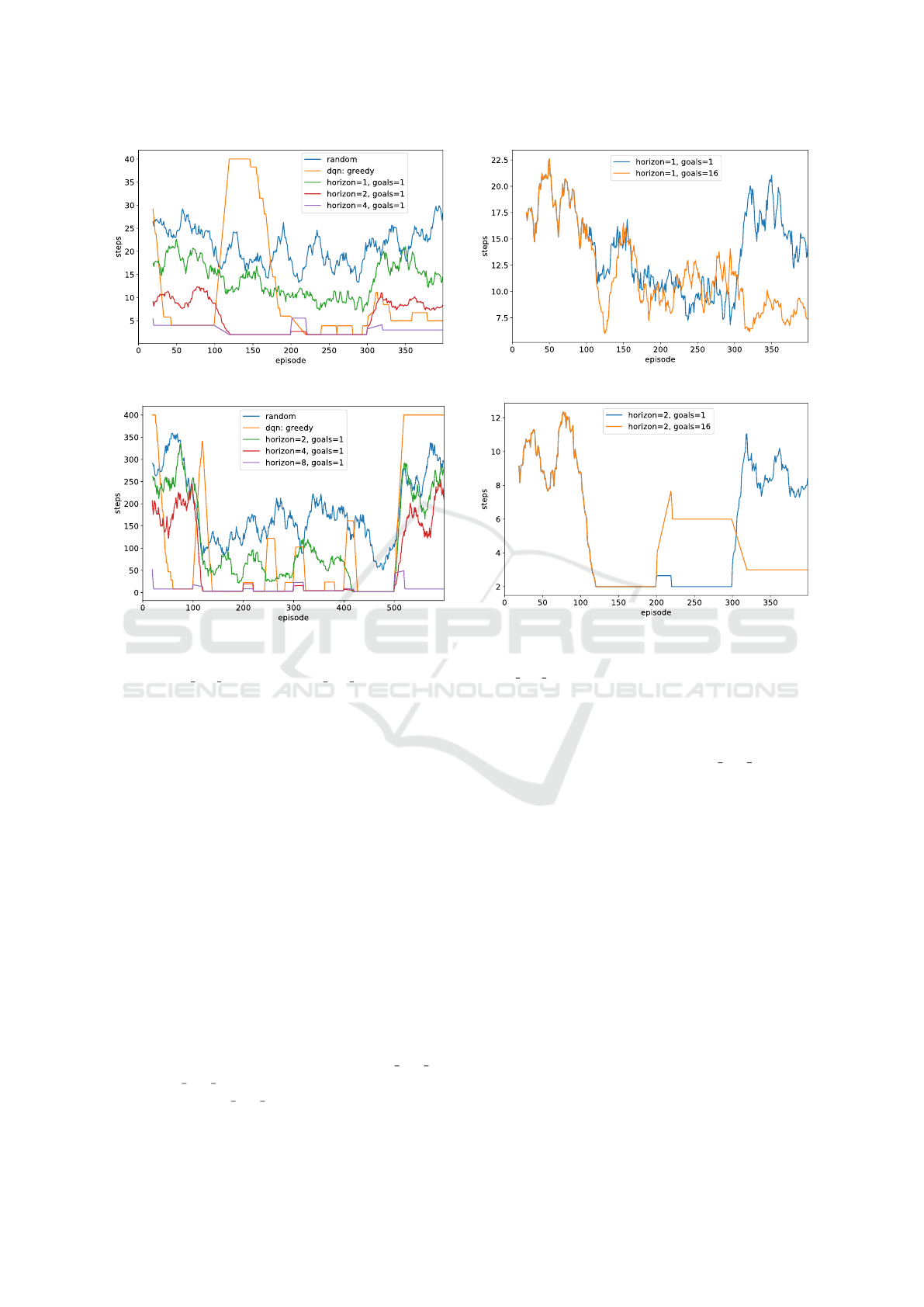
Figure 3: Episode durations (in steps) for handcrafted
mazes multi way v0 (a) and multi way v2 (b). Results
are shown with the moving average 20. Our agent per-
formed consistently better than pure random policy, and
with enough planning horizon it performed better than DQN
agent. Notice, how fast the agent with the planning horizon
8 learns an optimal path compared to the DQN agent.
vironment being changed every N
ep
episodes. We
compared our method’s performance with the base-
lines: random strategy and DQN ((Mnih et al., 2015)).
We also compared performance for different planning
horizons and the number of simultaneously tracked
goals in the goal tracking memory.
4.1 Experiments in Fixed Environments
This experiment setup was based on a number of
handcrafted mazes. Each experiment had a fixed
maze and the starting point s
0
, but the place of the re-
ward was being changed every N episodes. We tested
an agent’s ability to find the goal state and how it
adapts to the new goal position.
We present results for two mazes: multi
way v0
and multi way v2 (see Fig. 3 and Fig. 4). Each ex-
periment in multi way v0 had 4 different rewarding
goal positions being sequentially changed every 100
(a) Planning horizon H = 1
(b) Planning horizon H = 2
Figure 4: Episode durations (in steps) for the agent on
multi way v0 depending on how many rewarding goal
states it can track - last 16 or just the last one - grouped
by the planning horizon length. Results are shown with the
moving average 20.
episodes. Each experiment in multi way v2 had 6
rewarding goal positions being changed every 200
episodes. Schematic view of these mazes is provided
in Appendix 5.1.
In the tested environments our method performed
better than random policy. But the more complicated
an environment is the less distinctive is the difference
between the H = 0 and H = 1. Our method performs
better with the increase of the planning horizon H.
Each increment of the planning horizon is cumulative,
i.e. each next increment is more advantageous.
Regarding the goal tracking memory size, we
found that increase of the size leads to better explo-
ration. We think that’s because an agent less fre-
quently uses random strategy and therefore moves
less chaotically. However, sometimes this behavior
is suboptimal. For example when the rewarding goal
state is reachable from the current position in less than
H actions but there’s a fake goal state in the opposite
direction that is closer to the agent. We think that
these results are highly biased due to the special type
ICAART 2021 - 13th International Conference on Agents and Artificial Intelligence
1078

of handcrafted mazes and initial conditions.
We also found that an agent learns and adapts
faster than DQN agent (in terms of the number of
episodes required to steadily reach the goal during the
episode). And longer planning horizon leads to a bet-
ter adaptation to the changed rewarding position.
When the planning horizon is large enough to
reach the goal state from the starting position, then
the agent learns the optimal policy very fast. Accord-
ing to our experiments, in this case it learns approx-
imately 1.5-2.5 times faster than DQN. But for any
fixed planning horizon if we start rising an environ-
ment complexity, then at some point DQN starts to
perform better than our method. That’s because DQN
always finds an optimal path, and our agent finds it
only when it has enough planning horizon.
4.2 Experiments in Changing
Environments
In this experiment setup we used a number of ran-
domly generated GridWorld mazes of fixed size (see
Fig. 1). Each experiment has the following scheme.
Agent faces sequentially N
env
randomly generated
mazes. For a fixed maze the rewarding goal position
being changes sequentially N
rew
times. For a fixed re-
warding goal position the initial position changes se-
quentially N
s
0
times. And for a whole configuration
being fixed agent plays N episodes. Thus each experi-
ment has N
env
·N
rew
·N
s
0
·N episodes in total. We have
tested an agent’s ability not only to find the rewarding
goal and adapt to its new position, but also how the
agent adapts to the whole new maze.
We tested agent in mazes generated on 5 × 5, 6 ×
6 and 8 × 8 square grids. In this section we present
only the results for the 5 × 5 mazes, but for the other
tested sizes the results are similar. The key difference
in complexity of each experimental setup is the total
number of the episodes with fixed reward and maze.
The less episodes has agent to adapt, the more agile
it’s required to be.
We present results for the following experimental
setups:
1. Experimental setup with the rare change of re-
ward and maze: N
s
0
= 100, N
rew
= 2, N
env
= 8
(see Fig. 5)
2. Experimental setup with the frequent change of
reward and maze: N
s
0
= 20, N
rew
= 1, N
env
= 20
(see Fig. 6).
From this set of experiments we conclude that in av-
erage our agent adapts to changes faster than DQN.
Which also makes it perform more stable.
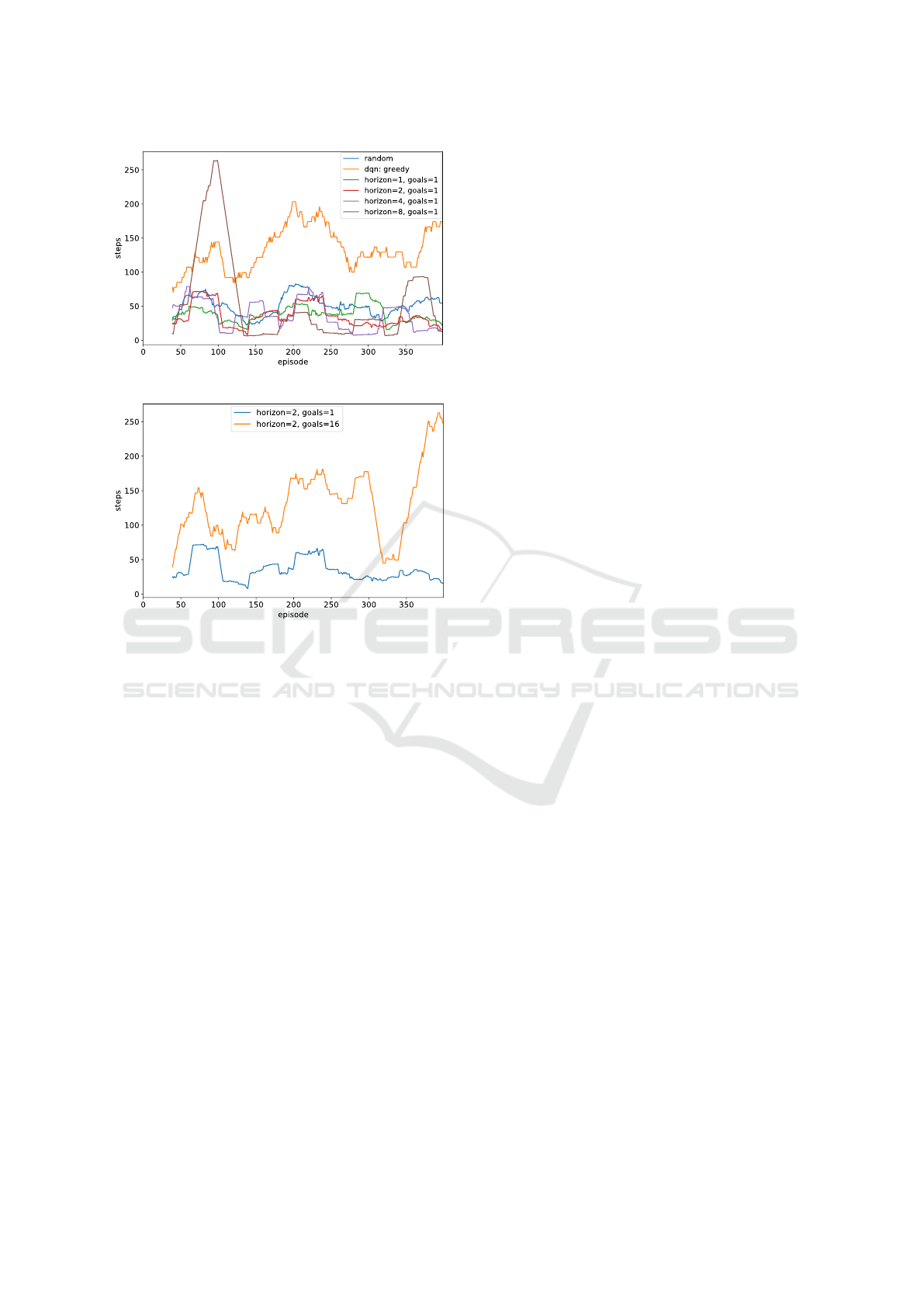
(a)
(b)
Figure 5: Episode durations for the experiment with rarely
changed environments. Results are shown with the moving
average 40. a) Comparison with the baselines. Our agent
with the planning horizon 8 performed the best. Notice,
how an each change of the environment configuration re-
sults in a spiked degradation of the performance for DQN
agent, while our agent quickly relearns new position. b)
Performance comparison for the different number of simul-
taneously tracked goals - the last goal or last 4; planning
horizon length = 2.
In contradiction to our results for the experiments in
the fixed handcrafted environments we found that the
increase of the number of the tracked goals makes our
method to perform worse.
5 CONCLUSIONS
We introduced a novel memory-based method that
combines learning the model of the environment with
the planning algorithm to infer a local policy. We
showed that under certain conditions (enough plan-
ning horizon) the resulting global policy is optimal or
at least very close to it. We also found that in such
cases, compared to DQN, our method learns with the
comparable speed or slightly faster in terms of the
Planning with Hierarchical Temporal Memory for Deterministic Markov Decision Problem
1079

(a)
(b)
Figure 6: Episode durations for the experiment with fre-
quently changed environments. Results are shown with the
moving average 40. a) Comparison with the baselines. Our
method performed more stable with small planning hori-
zons (1-4), while with planning horizon 8 it performed ei-
ther very good or very bad. DQN agent results were worse
than of random policy - the frequency of changes was too
high for it to adapt before the next change. b) Comparison
for the different number of simultaneously tracked goals;
planning horizon length = 2.
number of episodes required. The planning algorithm
with any non-zero planning horizon performs better
than random strategy. However, for the small plan-
ning horizons and hard tasks results are sufficiently
degraded and close to a pure random strategy.
To model the environment dynamics we used
human-like model of the memory called HTM. We
found that it’s capable to quickly and reliably learn
the transition model of the visited states in just a few
episodes. As far as we know it is the first time HTM
model was used for the model-based RL method. So,
even though we applied it to model very simple deter-
ministic environments with perfectly distinguishable
states the results are promising, and we look forward
to adapt our method to more complex environments.
Our experiments showed us that the naive scaling
of our method to environments with the larger state
space is limited due to limitations for planning hori-
zon increase. As for now we see two potential paths
to remedy this problem. The first is to learn the model
in a compact latent-space. The second is to make use
of hierarchical approach by building a hierarchy of
models and planners that operate in a different scales
of time and space. Also the fact that the backing up
strategy for a planner is purely random and not based
on the agent’s experience makes it a good target for
further improvements too.
ACKNOWLEDGEMENTS
The reported study was supported by RFBR, research
Projects No. 17-29-07051 and No. 18-29-22047.
REFERENCES
Berner, C., Brockman, G., Chan, B., Cheung, V., Debiak,
P., Dennison, C., Farhi, D., Fischer, Q., Hashme,
S., Hesse, C., Jozefowicz, R., Gray, S., Olsson, C.,
Pachocki, J., Petrov, M., de Oliveira Pinto, H. P.,
Raiman, J., Salimans, T., Schlatter, J., Schneider, J.,
Sidor, S., Sutskever, I., Tang, J., Wolski, F., and
Zhang, S. (2019). Dota 2 with large scale deep re-
inforcement learning.
Brown, N. and Sandholm, T. (2017). Superhuman ai for
heads-up no-limit poker: Libratus beats top profes-
sionals. Science, 359(6374):418–424.
Campbell, M., Hoane, A.Joseph, J., and Hsu, F.-h. (2002).
Deep blue. Artificial Intelligence, 134(1–2):57–83.
Coulom, R. (2007). Efficient Selectivity and Backup Op-
erators in Monte-Carlo Tree Search, page 72–83.
Springer Berlin Heidelberg.
Cui, Y., Ahmad, S., and Hawkins, J. (2017). The htm spa-
tial pooler—a neocortical algorithm for online sparse
distributed coding. Frontiers in Computational Neu-
roscience, 11.
Daylidyonok, I., Frolenkova, A., and Panov, A. I. (2019).
Extended Hierarchical Temporal Memory for Motion
Anomaly Detection. In Samsonovich, A. V., editor,
Biologically Inspired Cognitive Architectures 2018.
BICA 2018. Advances in Intelligent Systems and Com-
puting, volume 848, pages 69–81. Springer.
George, D. and Hawkins, J. (2009). Towards a mathemati-
cal theory of cortical micro-circuits. PLoS Computa-
tional Biology, 5(10):e1000532.
Gorodetskiy, A., Shlychkova, A., and Panov, A. I. (2020).
Delta Schema Network in Model-based Reinforce-
ment Learning. In Goertzel, B., Panov, A., Potapov,
A., and Yampolskiy, R., editors, Artificial General In-
telligence. AGI 2020. Lecture Notes in Computer Sci-
ence, volume 12177, pages 172–182. Springer.
Ha, D. and Schmidhuber, J. (2018). World models. Zenodo.
ICAART 2021 - 13th International Conference on Agents and Artificial Intelligence
1080

Haarnoja, T., Zhou, A., Abbeel, P., and Levine, S. (2018).
Soft actor-critic: Off-policy maximum entropy deep
reinforcement learning with a stochastic actor.
Hassabis, D., Kumaran, D., Summerfield, C., and
Botvinick, M. (2017). Neuroscience-inspired artificial
intelligence. Neuron, 95(2):245–258.
Hawkins, J. and Ahmad, S. (2016). Why neurons have thou-
sands of synapses, a theory of sequence memory in
neocortex. Frontiers in Neural Circuits, 10:23.
Kaiser, L., Babaeizadeh, M., Milos, P., Osinski, B., Camp-
bell, R. H., Czechowski, K., Erhan, D., Finn, C.,
Kozakowski, P., Levine, S., Mohiuddin, A., Sepassi,
R., Tucker, G., and Michalewski, H. (2020). Model-
based reinforcement learning for atari.
Mnih, V., Kavukcuoglu, K., Silver, D., Rusu, A. A., Veness,
J., Bellemare, M. G., Graves, A., Riedmiller, M., Fid-
jeland, A. K., Ostrovski, G., and et al. (2015). Human-
level control through deep reinforcement learning.
Nature, 518(7540):529–533.
Moerland, T. M., Broekens, J., and Jonker, C. M. (2020).
Model-based reinforcement learning: A survey.
Nugamanov, E. and Panov, A. I. (2020). Hierarchical Tem-
poral Memory with Reinforcement Learning. Proce-
dia Computer Science, 169:123–131.
Puterman, M. (1994). Markov Decision Processes. John
Wiley & Sons, Inc.
Schrittwieser, J., Antonoglou, I., Hubert, T., Simonyan, K.,
Sifre, L., Schmitt, S., Guez, A., Lockhart, E., Has-
sabis, D., Graepel, T., Lillicrap, T., and Silver, D.
(2020). Mastering atari, go, chess and shogi by plan-
ning with a learned model.
Schulman, J., Wolski, F., Dhariwal, P., Radford, A., and
Klimov, O. (2017). Proximal policy optimization al-
gorithms.
Silver, D., Huang, A., Maddison, C. J., Guez, A., Sifre, L.,
van den Driessche, G., Schrittwieser, J., Antonoglou,
I., Panneershelvam, V., Lanctot, M., Dieleman, S.,
Grewe, D., Nham, J., Kalchbrenner, N., Sutskever, I.,
Lillicrap, T., Leach, M., Kavukcuoglu, K., Graepel,
T., and Hassabis, D. (2016). Mastering the game of
go with deep neural networks and tree search. Nature,
529:484–503.
Skrynnik, A., Petrov, A., and Panov, A. I. (2016). Hierarchi-
cal Temporal Memory Implementation with Explicit
States Extraction. In Samsonovich, A. V., Klimov,
V. V., and Rybina, G. V., editors, Biologically Inspired
Cognitive Architectures (BICA) for Young Scientists.
Advances in Intelligent Systems and Computing, vol-
ume 449, pages 219–225. Springer.
APPENDIX
Handcrafted Mazes
The notation we use in the schematic views of the en-
vironments: - - empty cell, # - wall, @ - agent, X -
reward.
multi
way v0. Each experiment had 4 different re-
warding places being sequentially changed every 100
episodes:
##### ##### ##### #####
#@--# #@-X# #@--# #@--#
#-#-# #-#-# #-#-# #-#X#
#--X# #---# #X--# #---#
##### ##### ##### #####
multi way v2. Each experiment had 6 rewarding
places being changed every 200 episodes:
######### ######### #########
#---##### #-X-##### #---#####
#-#-##### #-#-##### #-#-#####
#--@---## #--@---## #--@--X##
###--#### ###--#### ###--####
###-#--X# ###-#---# ###-#---#
###---### ###---### ###---###
###-##### ###-##### ###-#####
######### ######### #########
######### ######### #########
#---##### #---##### #---#####
#-#-##### #-#-##### #-#-#####
#--@---## #X-@---## #--@---##
###--#### ###--#### ###--####
###-#---# ###-#---# ###-#--X#
###---### ###---### ###---###
###X##### ###-##### ###-#####
######### ######### #########
Planning with Hierarchical Temporal Memory for Deterministic Markov Decision Problem
1081