Autoencoder Watchdog Outlier Detection for Classiﬁers

Justin Bui and Robert J. Marks II

Department of Electrical and Computer Engineering, Baylor University, Waco, Texas, U.S.A.

Keywords:

Neural Networks, Watchdog, CNN, MNIST, Classiﬁer, Generator, Autoencoder.

Abstract:

Neural networks have often been described as black boxes. A generic neural network trained to differentiate

between kittens and puppies will classify a picture of a kumquat as a kitten or a puppy. An autoencoder

watchdog screens trained classiﬁer/regression machine input candidates before processing, e.g. to ﬁrst test

whether the neural network input is a puppy or a kitten. Preliminary results are presented using convolutional

neural networks and convolutional autoencoder watchdogs using MNIST images.

1 INTRODUCTION

Akin to principle component analysis (Oja, 1989), au-

toencoders can implicitly learn by the estimation of a

lower dimensional manifold on which training data

lives (Thompson et al., 2002; Thompson et al., 2003).

The feature space dimension is determined by the car-

dinality of the autoencoder’s input and output. The di-

mension of the manifold is dictated by the size of the

bottleneck layer (or waist) of the autoencoder. Repre-

sentative test data presented to a properly trained au-

toencoder will generate an output similar to the input.

More generally, the root mean square error

(RSME) between the autoencoder input and output

can be viewed as the rough distance measurement

between the autoencoder input and the training data

manifold in the feature space. For this reason, autoen-

coders can be used in novelty detection (Guttormsson

et al., 1999; Streifel et al., 1996; Thompson et al.,

2002).

One could train a neural network on three outputs:

kittens, puppies and all other images that are not kit-

tens or puppies. One challenge to this approach is that

the set of images that do not contain kittens or puppies

is prohibitively large. Work done by Abbasi and De-

Vries (Abbasi et al., 2019; DeVries and Taylor, 2018)

suggest strategies to work around the need for these

large datasets.

Use of an autoencoder watchdog is a more reason-

able solution (Streifel et al., 1996), acting as a nov-

elty (or anomaly) detector which protects the classi-

ﬁer neural network from fraudulent inputs. The au-

toencoder generates the manifold of data points that

represent kittens and puppies. Any image lying far

from the manifold is not a kitten or a puppy.

A data point that lies close to the manifold need

not be a kitten or a puppy. Another image may coin-

cidently lie on the manifold. In anomaly detection, a

ﬂag raised by the autoencoder is therefore sufﬁcient

for detecting anomalies but is not necessary for de-

tecting outliers.

2 BACKGROUND

Interest in, and the application of neural networks

(Reed and MarksII, 1999) continues to expand at a

rapid rate and cover a variety of tasks of varying com-

plexities. Yadav et al present an excellent introduction

to the history of neural networks (Yadav et al., 2015).

Autoencoder neural networks are of particular interest

in watchdog novelty detection. They have been used

in a variety of different applications and may be im-

plemented in a variety of different ways. For example,

Baur (Baur et al., 2018) has demonstrated anomaly

detection in medical scans, whereas Alvernaz (Alver-

naz and Togelius, 2017) explored the ability to visu-

ally analyze and learn to play complex videogames.

Vu (Vu et al., 2019) has investigated anomaly detec-

tion using adversarial autoencoders, while Lore (Lore

et al., 2017) has reported their use in low-light image

enhancement applications.

Autoencoders are useful for denoising various

types of data, from udio to medical images. Work

done by Gondara (Gondara, 2016) and Vincent (Vin-

cent et al., 2008) provide excellent examples of the

these denoising techniques. Autoencoders have been

also been used in generative networks, as described by

990

Bui, J. and Marks II, R.

Autoencoder Watchdog Outlier Detection for Classiﬁers.

DOI: 10.5220/0010300509900996

In Proceedings of the 13th International Conference on Agents and Artiﬁcial Intelligence (ICAART 2021) - Volume 2, pages 990-996

ISBN: 978-989-758-484-8

Mesheder (Mescheder et al., 2017). Most commonly

used in generative adversarial networks, or GANs,

autoencoders have shown remarkable capabilities in

generating images from noise. Work done by Zhifei

Zhang (Zhang et al., 2017), Zijun Zhang (Zhang et al.,

2020), Huang (Huang et al., 2018), and Ranjan (Ran-

jan et al., 2018) have shown some impressive gen-

erative capabilities across multiple spectrums, from

grayscale digits to 3D face images. Work done by

Luo (Luo et al., 2017) demonstrates different tech-

niques based on the combination of variational au-

toencoders (VAEs) and GANs. Work done by Lu (Lu

et al., 2013), Xia (Xia et al., 2014), and Qi (Qi et al.,

2017) have demonstrated various applications beyond

denoising and generation, highlighting the ﬂexibility

and useability of autoencoders.

As the artiﬁcial neural network ﬁeld continues to

grow and new tools continue to be developed, it is be-

coming easier to develop neural networks without a

deep understanding of the driving principles. These

new tools (eg TensorFlow, PyTorch, Keras, FastAI)

lead to many neural networks being generally treated

as black boxes. Our interest in these black boxes, as

described by Alain et al (Alain and Bengio, 2016),

is less aimed at diving into the inner workings and

attempting to demystify them, but rather to develop

a technique that may be used with both existing and

newly developed neural networks to address the un-

certainty born of opaque neural networks. While there

have been several attempts at diving in to the under-

standing of neural networks, such as the work done

by Schartz (Shwartz-Ziv and Tishby, 2017), Zeiler

(Zeiler and Fergus, 2014), Martin (Martın-Clemente

and Zarzoso, 2016) and Markopoulos (Markopoulos

et al., 2017), much of today’s end products are as-

sumed to be “black boxes”.

While there is no shortage of neural network struc-

tures and applications, our research focuses on convo-

lutional neural networks (CNN’s) and autoencoders.

CNN’s have demonstrated impressive performance in

the classiﬁcation and generation of data. As an exam-

ple, Zhang (Zhang and LeCun, 2015) provides an ex-

cellent introduction to the concept of text understand-

ing, paralleling the interpretation of hand written dig-

its. Bhatnagar (Bhatnagar et al., 2017) demonstrates

the classiﬁcation capabilities of CNNs on clothing

items. Other work (Ciresan et al., 2011; Tabik et al.,

2017) further details these capabilities while introduc-

ing new approaches for network design and perfor-

mance optimization.

3 THE NEURAL NETWORK

WATCHDOG

The Neural Network Watchdog is a tool to determine

a neural network’s output validity. This is achieved

by using the generative component of the autoencoder

to reconstruct the input data and calculating a differ-

ence score. The difference score is then compared

to a threshold that determines data validity. In this

paper, we build on the use of autoencoders to create

the generative component of the watchdog. For our

differencing component, the root mean square error

(RMSE: the square root of the sum of the squares)

is calculated and comparing against a ﬁxed thresh-

old. Below are descriptions of the classiﬁcation

and watchdog autoencoder networks, the training and

evaluation datasets, and the classiﬁer and watchdog

performance analysis.

3.1 Network Structures

For the viability study, both our classiﬁer and autoen-

coder are CNN’s. Work by LeCun (LeCun et al.,

2015), Ng (Ng et al., 2011), and Meng (Meng et al.,

2017) provide an excellent foundation for designing

such networks. The MNIST handwritten digit im-

age dataset is used to train the neural network and its

watchdog autoencoder.

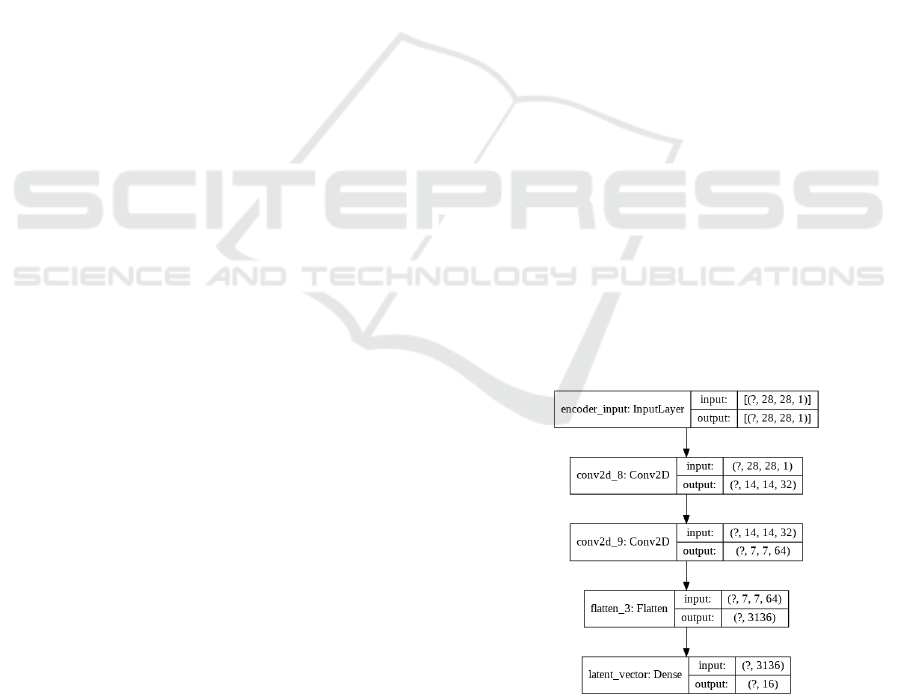
3.1.1 The Autoencoder Watchdog

The CNN autoencoder is comprised of a convolu-

tional encoder network, coupled with a decoding net-

work. The encoder structure is shown in Figure. 1.

Figure 1: The encoder is comprised of two 2D convolution

layers, one ﬂatten layer, and one dense layer. This produces

a lower dimension representation of the input data.

The decoding structure mirrors the encoder structure,

as shown in Figure. 2. The encoder and decoder struc-

Autoencoder Watchdog Outlier Detection for Classiﬁers

991

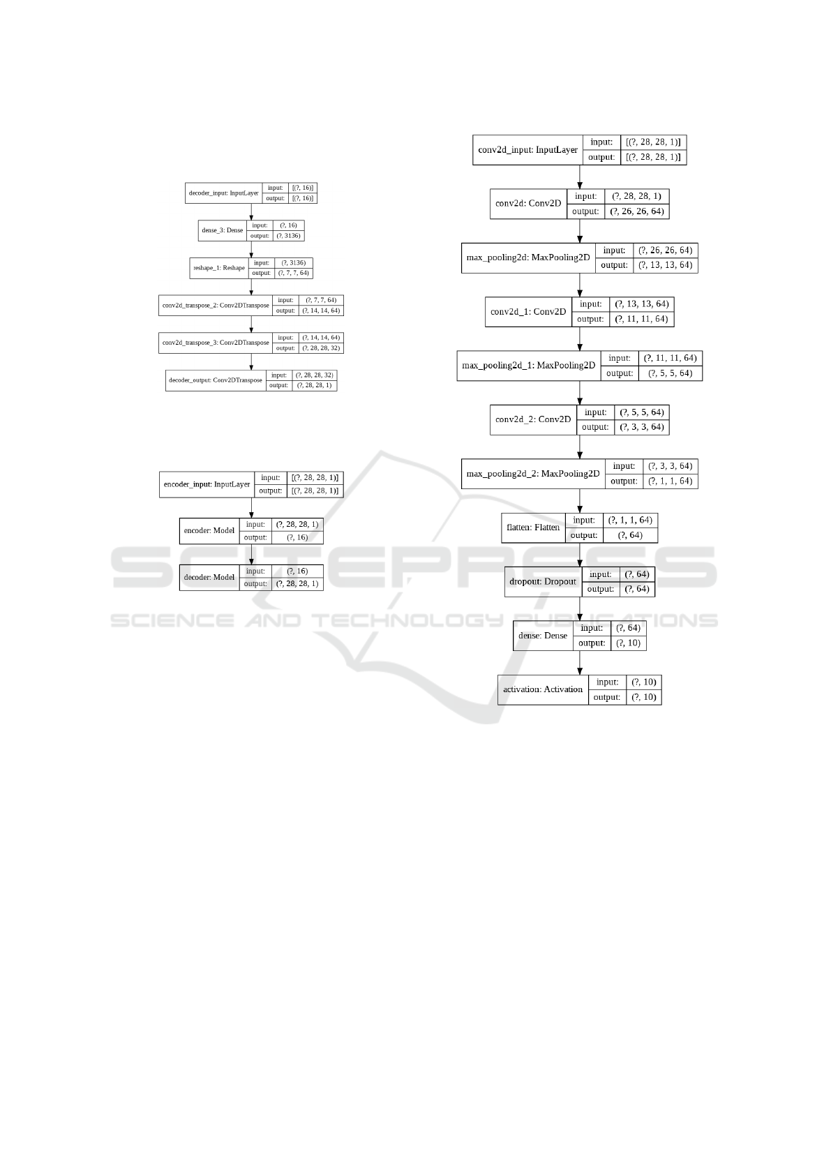
tures are stacked to form the autoencoder. The result-

ing structure is shown in Figure. 3.

Figure 2: The decoder, which mirrors the encoder network.

By matching the encoder’s structure, the decoder can repro-

duce data structurally identical to the encoder input using

the lower dimension representation created by the encoder.

Figure 3: The autoencoder, comprised of the encoder and

decoder, allows the watchdog to generate input data based

on the representations created at the waist layer.

3.1.2 Convolutional Neural Network Structure

As demonstrated by Ciresan (Ciresan et al., 2011),

Tabik (Tabik et al., 2017), and Bhatnagar (Bhatna-

gar et al., 2017), CNNs have shown impressive image

classiﬁcation capabilities. Our convolutional neural

network classiﬁer, described in Figure 4, is modeled

after an example CNN provided by Geron in (G

eron,

2019).

3.2 Training the Networks

3.2.1 Training and Evaluation Datasets

With the structures of the networks established,

we turn to identifying the training and evaluation

datasets. The training data comes entirely from the

MNIST handwritten digit dataset, and consists of

60,000 training and 10,000 test images evenly split

across 10 classes of digits, 0-9. The evaluation dataset

is augmented to include the fashion MNIST dataset

Figure 4: Classiﬁcation convolutional neural network struc-

ture, comprised of 3 Layers of 2D convolutions paired with

2D max pooling, one ﬂatten layer, and one dropout layer,

with a softmax activation layer.

test images. First introduced by Xiao in 2017 (Xiao

et al., 2017), the fashion MNIST dataset is comprised

of 70,000 total images, evenly distributed across 10

classes of different clothing types. These datasets

were chosen due to their identical size, allowing for

their easy use in the training and testing of both the

autoencoder and classiﬁer without modiﬁcation. Both

the autoencoder and the CNN were trained on 50,000

digit image dataset and validated on an additional

10,000 digit images from the training set. Examples

of the training data are shown in Figures. 5a and 5b.

In order to evaluate the effectiveness of the clas-

siﬁer and its watchdog, three evaluation datasets are

used. The evaluation datasets are the combination of

ICAART 2021 - 13th International Conference on Agents and Artiﬁcial Intelligence

992

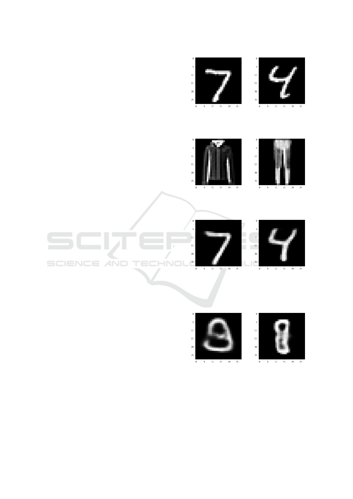
test images from the digit and fashion image sets. Ad-

ditional examples can be seen in Figures. 6a and 6b.

Note that the evaluation images are separate from the

training and validation datasets. The three datasets

are as follows: in-distribution (digit images), out-of-

distribution (fashion images), and mixed-distribution

(both digit and fashion images).

1. 10,000 test images from the MNIST digit dataset,

in-distribution data

2. 10,000 test images from the fashion MNIST

dataset, out-of-distribution data

3. 20,000 test images resulting from the combina-

tion of the MNIST digit and fashion MNIST test

datasets, mixed-distribution data

4 EVALUATING THE

NETWORKS

4.1 Evaluating the Autoencoder

With the three evaluation datasets established, the

performance of the autoencoder is examined. The

MNIST digit and fashion MNIST datasets are passed

through the autoencoder independently. The outputs

of the autoencoder, examples of which can be seen

in Figures. 7a, 7b, 8a, and 8b, were then stored sepa-

rately for additional analysis. The resulting generated

images were then compared to their respective origi-

nal images and the RMSE was calculated. In order to

determine the range of values expected when calculat-

ing the RMSE, multiply the image size, 28x28x1 pix-

els, by the maximum pixel value, which has been nor-

malized to values between 0 and 1. For this dataset,

the range of RMSE values is between 0 and 28, with a

RMSE of 0 representing a perfect match, and a RMSE

of 28 representing a perfect mismatch. Based on our

experimentation, the average RMSE value calculated

for the MNIST digit dataset was approximately 2.4,

and the average RMSE value calculated for the fash-

ion MNIST dataset was approximately 7.9.

4.2 Performance of the Watchdog

4.2.1 ROC Curves and Classiﬁcation Errors

In order to show the effectiveness of the watchdog,

we produce receiver operator characteristic (ROC)

curves. These curve show the tradeoff between the

true positive vs. false positive rates. The rates are

determined as:

(a) An example of the

MNIST digit 7

(b) An example of the

MNIST digit 4

Figure 5: MNIST digit image examples.

(a) An example of the fash-

ion MNIST jacket class

(b) An example of the fash-

ion MNIST pants class

Figure 6: Fashion MNIST image examples.

(a) Watchdog regeneration

of the in-distribution digit

(b) Watchdog regeneration

of the in-distribution digit

Figure 7: Watchdog autoencoder regeneration of the in-

distribution MNIST digit images.

(a) Watchdog regeneration

of the out-of-distribution

jacket image.

(b) Watchdog regeneration

of the out-of-distribution

pants image

Figure 8: Watchdog autoencoder regeneration of the out-of-

distribution fashion MNIST images.

T PR = T P/(T P + FN) (1)

FPR = FP/(FP + T N) (2)

Autoencoder Watchdog Outlier Detection for Classiﬁers

993

where:

• TP - True Positive = correct classiﬁcation, the in-

distribution inputs that are within the acceptance

threshold

• FP - False Positive = incorrect classiﬁcation, the

out-of-distribution inputs are within the accep-

tance threshold

• FN - False Negative = incorrect classiﬁcation,

the out-of-distribution inputs are above the accep-

tance threshold

• TN - True Negative = correct classiﬁcation, the

in-distribution inputs are above the acceptance

threshold

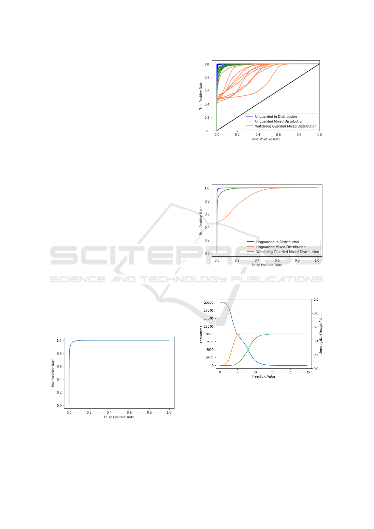
With the average RMSE values established, the next

step is determining an appropriate threshold. Fig-

ure. 9 shows the ROC curve for the watchdog autoen-

coder. This curve is the evaluation of the watchdog

autoencoder based on its ability to separate the in-

distribution digit images, or true positives, from out-

of-distribution fashion images, or false positives.

4.2.2 Monitoring the Classiﬁer with the

Watchdog Autoencoder

The value of adding the autoencoder watchdog to

the mixed-distribution dataset can be seen in Fig-

ure. 10 where the guarded mixed-distribution dataset

has better performance than the unguarded mixed-

distribution. As a point of reference, the ideal

scenario, data contained only in the in-distribution

dataset, has been included in Figure. 10. As we have

shown, the results from the watchdog produce a more

accurate true positive vs. false positive rate, and a

more vertical ROC curve, when compared to the indi-

vidual dataset performance.

Figure 9: The ROC plot showing the performance of the

watchdog using the mixed-distribution dataset. This curve

has been produced based on the watchdog’s ability to differ-

entiate between in-distribution and out-of-distribution data

as a function of RMSE threshold.

Figure 10: The ROC plots showing the watchdog perfor-

mance on the three evaluation datasets. Blue indicates un-

guarded in-distribution performance, Orange indicates un-

guarded mixed-distribution performance, and Green indi-

cates guarded mixed-distribution performance.

Figure 11: The averaged ROC plots of the unguarded

in-distribution, unguarded mixed-distribution, and guarded

mixed-distribution plots, as seen in Figure. 10 above.

Figure 12: The distribution of images as a function of

RMSE threshold. Blue represents unrecognized images

(images that exceed RMSE threshold), orange represents in-

distribution images (True Positives), and green represents

out-of-distribution images (False Positives).

Along with the ROC curves, an interesting metric to

note is the number of unrecognized images that have

been detected in the dataset. The number of unrec-

ognized images and the unrecognized image ratio, as

ICAART 2021 - 13th International Conference on Agents and Artiﬁcial Intelligence

994

seen in Figure. 12, can be used as tools to help de-

termine a ﬁnal threshold value when designing and

developing watchdog guarded networks.

5 CONCLUSION

An initial proof of concept neural network watch-

dog is proposed to help improve the performance

of classiﬁers on various datasets. The approach is

also transparently applicable to regression neural net-

works. The choice of RMSE threshold is ultimately

determined by the desired detection versus false alarm

tradeoff. Alternately, the RMSE can be used to in-

form users of a measure of closeness of an input to

the manifold of the watchdog autoencoder deﬁned in-

distribution manifold in feature space.

REFERENCES

Abbasi, M., Shui, C., Rajabi, A., Gagne, C., and Bobba,

R. (2019). Toward metrics for differentiating out-of-

distribution sets. arXiv preprint arXiv:1910.08650.

Alain, G. and Bengio, Y. (2016). Understanding intermedi-

ate layers using linear classiﬁer probes. arXiv preprint

arXiv:1610.01644.

Alvernaz, S. and Togelius, J. (2017). Autoencoder-

augmented neuroevolution for visual doom playing.

In 2017 IEEE Conference on Computational Intelli-

gence and Games (CIG), pages 1–8. IEEE.

Baur, C., Wiestler, B., Albarqouni, S., and Navab, N.

(2018). Deep autoencoding models for unsupervised

anomaly segmentation in brain mr images. In Inter-

national MICCAI Brainlesion Workshop, pages 161–

169. Springer.

Bhatnagar, S., Ghosal, D., and Kolekar, M. H. (2017).

Classiﬁcation of fashion article images using convolu-

tional neural networks. In 2017 Fourth International

Conference on Image Information Processing (ICIIP),

pages 1–6. IEEE.

Ciresan, D. C., Meier, U., Masci, J., Gambardella, L. M.,

and Schmidhuber, J. (2011). Flexible, high perfor-

mance convolutional neural networks for image clas-

siﬁcation. In Twenty-second international joint con-

ference on artiﬁcial intelligence.

DeVries, T. and Taylor, G. W. (2018). Learning conﬁdence

for out-of-distribution detection in neural networks.

arXiv preprint arXiv:1802.04865.

eron, A. (2019). Hands-on machine learning with Scikit-

Learn, Keras, and TensorFlow: Concepts, tools, and

techniques to build intelligent systems. O’Reilly Me-

dia.

Gondara, L. (2016). Medical image denoising using convo-

lutional denoising autoencoders. In 2016 IEEE 16th

International Conference on Data Mining Workshops

(ICDMW), pages 241–246. IEEE.

Guttormsson, S. E., Marks, R., El-Sharkawi, M., and Ker-

szenbaum, I. (1999). Elliptical novelty grouping for

on-line short-turn detection of excited running rotors.

IEEE Transactions on Energy Conversion, 14(1):16–

22.

Huang, H., He, R., Sun, Z., Tan, T., et al. (2018). In-

trovae: Introspective variational autoencoders for pho-

tographic image synthesis. In Advances in neural in-

formation processing systems, pages 52–63.

LeCun, Y., Bengio, Y., and Hinton, G. (2015). Deep learn-

ing. nature, 521(7553):436–444.

Lore, K. G., Akintayo, A., and Sarkar, S. (2017). Llnet: A

deep autoencoder approach to natural low-light image

enhancement. Pattern Recognition, 61:650–662.

Lu, X., Tsao, Y., Matsuda, S., and Hori, C. (2013). Speech

enhancement based on deep denoising autoencoder. In

Interspeech, volume 2013, pages 436–440.

Luo, J., Xu, Y., Tang, C., and Lv, J. (2017). Learning inverse

mapping by autoencoder based generative adversarial

nets. In International Conference on Neural Informa-

tion Processing, pages 207–216. Springer.

Markopoulos, P. P., Kundu, S., Chamadia, S., and Pados,

D. A. (2017). Efﬁcient l1-norm principal-component

analysis via bit ﬂipping. IEEE Transactions on Signal

Processing, 65(16):4252–4264.

Martın-Clemente, R. and Zarzoso, V. (2016). On the link

between l1-pca and ica. IEEE transactions on pattern

analysis and machine intelligence, 39(3):515–528.

Meng, Q., Catchpoole, D., Skillicom, D., and Kennedy, P. J.

(2017). Relational autoencoder for feature extraction.

In 2017 International Joint Conference on Neural Net-

works (IJCNN), pages 364–371. IEEE.

Mescheder, L., Nowozin, S., and Geiger, A. (2017). Ad-

versarial variational bayes: Unifying variational au-

toencoders and generative adversarial networks. arXiv

preprint arXiv:1701.04722.

Ng, A. et al. (2011). Sparse autoencoder. CS294A Lecture

notes, 72(2011):1–19.

Oja, E. (1989). Neural networks, principal components, and

subspaces. International journal of neural systems,

1(01):61–68.

Qi, Y., Shen, C., Wang, D., Shi, J., Jiang, X., and Zhu, Z.

(2017). Stacked sparse autoencoder-based deep net-

work for fault diagnosis of rotating machinery. Ieee

Access, 5:15066–15079.

Ranjan, A., Bolkart, T., Sanyal, S., and Black, M. J. (2018).

Generating 3d faces using convolutional mesh autoen-

coders. In Proceedings of the European Conference

on Computer Vision (ECCV), pages 704–720.

Reed, R. and MarksII, R. J. (1999). Neural smithing: su-

pervised learning in feedforward artiﬁcial neural net-

works. Mit Press.

Shwartz-Ziv, R. and Tishby, N. (2017). Opening the black

box of deep neural networks via information. arXiv

preprint arXiv:1703.00810.

Streifel, R. J., Marks, R., El-Sharkawi, M., and Kerszen-

baum, I. (1996). Detection of shorted-turns in the

ﬁeld winding of turbine-generator rotors using novelty

detectors-development and ﬁeld test. IEEE Transac-

tions on Energy Conversion, 11(2):312–317.

Autoencoder Watchdog Outlier Detection for Classiﬁers

995

Tabik, S., Peralta, D., Herrera-Poyatos, A., and Herrera, F.

(2017). A snapshot of image pre-processing for con-

volutional neural networks: case study of mnist. Inter-

national Journal of Computational Intelligence Sys-

tems, 10(1):555–568.

Thompson, B. B., Marks, R., and El-Sharkawi, M. A.

(2003). On the contractive nature of autoencoders:

Application to missing sensor restoration. In Proceed-

ings of the International Joint Conference on Neural

Networks, 2003., volume 4, pages 3011–3016. IEEE.

Thompson, B. B., Marks, R. J., Choi, J. J., El-Sharkawi,

M. A., Huang, M.-Y., and Bunje, C. (2002). Im-

plicit learning in autoencoder novelty assessment. In

Proceedings of the 2002 International Joint Con-

ference on Neural Networks. IJCNN’02 (Cat. No.

02CH37290), volume 3, pages 2878–2883. IEEE.

Vincent, P., Larochelle, H., Bengio, Y., and Manzagol, P.-

A. (2008). Extracting and composing robust features

with denoising autoencoders. In Proceedings of the

25th international conference on Machine learning,

pages 1096–1103.

Vu, H. S., Ueta, D., Hashimoto, K., Maeno, K., Pranata,

S., and Shen, S. M. (2019). Anomaly detection

with adversarial dual autoencoders. arXiv preprint

arXiv:1902.06924.

Xia, R., Deng, J., Schuller, B., and Liu, Y. (2014). Model-

ing gender information for emotion recognition using

denoising autoencoder. In 2014 IEEE International

Conference on Acoustics, Speech and Signal Process-

ing (ICASSP), pages 990–994. IEEE.

Xiao, H., Rasul, K., and Vollgraf, R. (2017). Fashion-

mnist: a novel image dataset for benchmark-

ing machine learning algorithms. arXiv preprint

arXiv:1708.07747.

Yadav, N., Yadav, A., and Kumar, M. (2015). History of

neural networks. In An Introduction to Neural Net-

work Methods for Differential Equations, pages 13–

15. Springer.

Zeiler, M. D. and Fergus, R. (2014). Visualizing and under-

standing convolutional networks. In European confer-

ence on computer vision, pages 818–833. Springer.

Zhang, X. and LeCun, Y. (2015). Text understanding from

scratch. arXiv preprint arXiv:1502.01710.

Zhang, Z., Song, Y., and Qi, H. (2017). Gans powered by

autoencoding a theoretic reasoning. In ICML Work-

shop on Implicit Models.

Zhang, Z., Zhang, R., Li, Z., Bengio, Y., and Paull, L.

(2020). Perceptual generative autoencoders. In In-

ternational Conference on Machine Learning, pages

11298–11306. PMLR.

ICAART 2021 - 13th International Conference on Agents and Artiﬁcial Intelligence

996