TrajNet: An Efﬁcient and Effective Neural Network

for Vehicle Trajectory Classiﬁcation

Jiyong Oh, Kil-Taek Lim and Yun-Su Chung

Daegu-Gyeongbuk Research Center, Electronics and Telecommunications Research Institute (ETRI), Daegu, Korea

Keywords:

Vehicle Trajectory Classiﬁcation, TrajNet, Deep Neural Network, Intelligent Transportation System.

Abstract:

Vehicle trajectory classiﬁcation plays an important role in intelligent transportation systems because it can be

utilized in trafﬁc ﬂow estimation at an intersection and anomaly detection such as trafﬁc accidents and viola-

tions of trafﬁc regulations. In this paper, we propose a new neural network architecture for vehicle trajectory

classiﬁcation by modifying the PointNet architecture, which was proposed for point cloud classiﬁcation and

semantic segmentation. The modiﬁcations are derived based on analyzing the differences between the prop-

erties of vehicle trajectory and point cloud. We call the modiﬁed network TrajNet. It is demonstrated from

experiments using three public datasets that TrajNet can classify vehicle trajectories faster and more slightly

accurate than the conventional networks used in the previous studies.

1 INTRODUCTION

Smart city is one of the important convergence tech-

nologies that need to be developed to improve the

quality of human life. Intelligent transportation sys-

tem (ITS) is a representative technology required

in smart city, which makes it possible for people

to use road trafﬁc networks safely and efﬁciently

through real-time monitoring and effective trafﬁc con-

trol. Since vehicle trajectory has essential information

about movement direction and speed of vehicles, it

can be used in trafﬁc ﬂow estimation (Lv et al., 2015)

and trafﬁc anomaly detection (Zhao et al., 2019),

which are typical applications of ITS. In this study,

we focus on classifying those vehicle trajectories ex-

tracted by tracking vehicles as in (Ren et al., 2018).

Trajectory classiﬁcation or clustering has been

studied in various applications such as behavior anal-

ysis (Wang et al., 2008), group detection (Li et al.,

2017), semantic region analysis (Wang et al., 2011),

and trafﬁc vedio surveillence (Morris and Trivedi,

2009), (Hu et al., 2013), (Lin et al., 2017). In

early studies, researchers were mainly interested in

the mathematical representation of trajectories and

the similarity measure between them. In (Porikli,

2004), the authors proposed a new similarity measure

based on the hidden Markov model, and in (Morris

and Trivedi, 2009), six similarity measures were com-

pared and evaluated for trajectory clustering. Also,

in (Hu et al., 2013), the Dirichlet process mixture

model (DPMM) was employed for trajectory analy-

sis such as clustering, modeling, and retrieval. An

incremental method using DPMM was developed to

automatically determine the number of clusters, and

a time-sensitive DPMM was also proposed to en-

code the time-dependent characteristics of trajecto-

ries. In (Xu et al., 2015), an effective and robust

trajectory clustering method was proposed based on

shrinking trajectories. The method consists of an

adaptive multi-kernel estimation process and an op-

timization process. The adaptive multi-kernel estima-

tion process was employed to reduce intra-variation

and enlarge inter-variation between trajectories. And,

the optimization process with speed regularization

was introduced to utilize the shape information of the

original trajectory and the discriminative information

obtained from the estimation based on the adaptive

multi-kernels. Moreover, in (Lin et al., 2017), the

authros presented a novel representation based on a

three-dimensional tube and a droplet process. Given

a set of trajectories, a thermal transfer ﬁeld was con-

structed to capture global information of the trajecto-

ries, and a three-dimensional tube was generated from

each trajectory using the relation between its points

and the thermal transfer ﬁeld. Then, the droplet-based

process was applied to provide a low dimensional

droplet vector that encodes the high dimensional in-

formation in the three-dimensional tube.

After the impressive successes of deep neural net-

works such as (Krizhevsky et al., 2012) and (Ren

408

Oh, J., Lim, K. and Chung, Y.

TrajNet: An Efﬁcient and Effective Neural Network for Vehicle Trajectory Classiﬁcation.

DOI: 10.5220/0010243304080416

In Proceedings of the 10th International Conference on Pattern Recognition Applications and Methods (ICPRAM 2021), pages 408-416

ISBN: 978-989-758-486-2

et al., 2015), deep learning-based approaches have

been applied in many studies of various applications

such as human activity recognition (Yang et al., 2015)

and GPS trajectory analysis (Jiang et al., 2017), (Yao

et al., 2017), (Song et al., 2018). In (Yang et al.,

2015), by applying a sliding window, time-series sig-

nals captured by multiple sensors split into a set of

short intervals of multiple signals. The short inter-

vals were represented as two-dimensional matrices

corresponding to the input of a convolutional neu-

ral network (CNN) to solve human activity recogni-

tion problems. In (Jiang et al., 2017), a new method,

TrajectoryNet, was proposed to detect human trans-

portation mode using GPS trajectory. The proposed

method extracted the segment-based features and the

point-based features from GPS data. Then, the fea-

tures of different types were combined and classi-

ﬁed using an RNN based on the bidirectional maxout

gated recurrent units (GRUs). In (Yao et al., 2017), a

deep learning-based representation of trajectory was

presented. In the study, a feature sequence was gen-

erated from a trajectory using a sliding window tech-

nique, and it was transformed into a deep representa-

tion with a ﬁxed-size by a sequence-to-sequence au-

toencoder. The representation was applied in cluster-

ing and analyzing GPS trajectories. In (Song et al.,

2018), taxi fraud detection was addressed using GPS

trajectories. The long short term memory (LSTM)

and GRU cells were utilized in RNN to solve the

problem.

On the other hand, deep neural networks were also

applied in trafﬁc video surveillance (Ma et al., 2018),

(Santhosh et al., 2018). In (Ma et al., 2018), trajectory

distance metrics were presented to measure similari-

ties and detect anomalous trajectories, and an RNN-

based autoencoder was used in computing the met-

rics. Also, two different deep neural networks were

used in (Santhosh et al., 2018). In the method, a CNN

classiﬁes an input trajectory converted into an image

using the gradient conversion method, and a varia-

tional autoencoder decides whether the input trajec-

tory image is an anomaly or not.

In this paper, we propose a deep neural network

architecture to address the vehicle trajectory classiﬁ-

cation. Inspired from PointNet (Qi et al., 2017) that

is a novel neural network proposed for classiﬁcation

or semantic segmentation of point cloud data, the pro-

posed architecture is derived based on analyzing the

differences between the characteristics of point cloud

and trajectory. We call the new architecture Tra-

jNet. To our best knowledge, this is the ﬁrst study us-

ing the other network for vehicle trajectory classiﬁca-

tion instead of the conventional neural networks such

as RNN, LSTM, and CNN. We demonstrate by per-

forming experiments that the proposed method yields

slightly better classiﬁcation performances compared

to the conventional architectures like a vanilla RNN

and an RNN with LSTM unit as well as the CNN with

the gradient conversion method proposed for vehi-

cle trajectory classiﬁcation in (Santhosh et al., 2018).

Furthermore, it is also shown that the proposed net-

work can classify a trajectory faster than those net-

works.

This paper is organized as follows. In the next

section, a preprocessing method is explained together

with the conventional networks which have been pre-

viously presented for the vehicle or GPS trajectory

classiﬁcation. The proposed network architecture is

described in Sec. 3. Then, we verify in Sec. 4 that the

proposed network is more effective and efﬁcient than

the other networks employed in the previous studies

for the trajectory classiﬁcation. Finally, we conclude

this paper in the last section.

2 PRELIMINARIES

2.1 Preprocessing

One of the difﬁculties in using a trajectory as an input

of neural networks is the fact that the number of points

included in it is not the same. To input an arbitrary

trajectory to a neural network, which has a regular in-

put structure, we generate the input trajectory with M

points using the cubic B-spline curves approximation

as in (Ma et al., 2018). Figure 1 shows an original tra-

jectory and the trajectories generated by the method

when M = 16, M = 32, and M = 64. In the ﬁgure,

each point in trajectories is represented as a marker

located at its coordinates on the image. The color of

the points is determined by the gradient conversion

(Santhosh et al., 2018), in which the hue value h of

the i-th point p

in a trajectory T = {p

= (x

, y

)}

i=1

is computed as

h(p

) =

× 180.

The other two values of the HSV color model are set

to 255. We can see from the ﬁgure that each trajectory

can be normalized to have a ﬁxed number of points by

the cubic B-spline curves approximation method.

Each point in a trajectory can have its time step as p

, y

, t

), but we do not consider those time steps in this

study.

TrajNet: An Efﬁcient and Effective Neural Network for Vehicle Trajectory Classiﬁcation

409

(a) Original (b) M = 16 (c) M = 32 (d) M = 64

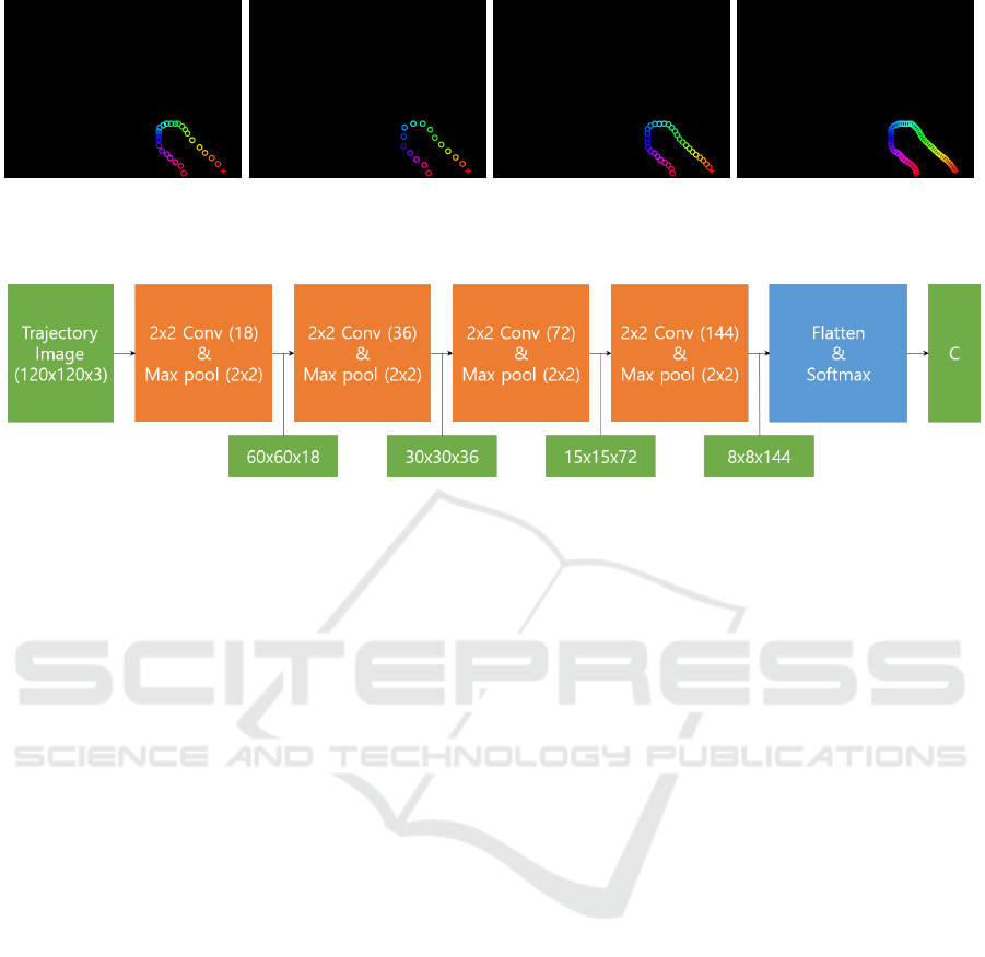
Figure 1: An original trajectory with M = 26 and the trajectories generated by the normalization based on the cubic B-spline

curves approximation. Best viewed in color.

Figure 2: The architecture of CNN used in this study.

2.2 RNN and LSTM

RNN is a kind of neural network suitable for process-

ing sequential data (Goodfellow et al., 2016). Since

a vehicle trajectory is a sequence of ordered points,

it is straightforward to apply an RNN to the vehicle

trajectory classiﬁcation. For this reason, we ﬁrst con-

sider a stacked RNN, and the number of the stacked

RNN layers is set to 3 based on experiments. In each

layer of the stacked RNN, the hyperbolic tangent ac-

tivation function is employed in its 128-dimensional

hidden state. The stacked RNN is connected to an ad-

ditional fully-connected layer with the sigmoid acti-

vation function, and the dimension of the hidden layer

in the fully-connected layer is also set to 128. Fi-

nally, the softmax layer follows the fully-connected

layer for C-class classiﬁcation. After the normaliza-

tion described in the previous subsection, each point

in a trajectory is input to the stacked RNN at a time,

and for the trajectory, the stacked RNN provides the

C-dimensional vector, each component of which cor-

responds to the probabilities belonging to each class.

However, it is well known that the conventional

RNN has the vanishing gradient problem, which de-

teriorates its learning capability when the length of

sequence data is longer. In order to alleviate the prob-

lem, the LSTM cell has been popularly used instead

of the original RNN cell in practice. Thus, we also

consider another RNN using the LSTM cells as in

(Song et al., 2018) together with the conventional

RNN. The LSTM-based RNN has the same architec-

ture as the stacked RNN mentioned above except for

using the LSTM cell. The two RNNs mentioned in

this subsection will be applied in the vehicle trajec-

tory classiﬁcation and compared to the different types

of neural networks mentioned later in Sec. 4.

2.3 CNN

CNN was originally developed to classify image data

with a type of grid. Since its remarkable successes in

image classiﬁcation (Krizhevsky et al., 2012), it has

become very popular in various ﬁelds. However, to

classify a trajectory using a CNN, it should have a reg-

ular form with a pre-determined size such as an im-

age. We convert each trajectory into an image shown

in Fig. 1. Then, the generated image is input to the

CNN proposed in (Santhosh et al., 2018). In the im-

age generation, we employ the gradient conversion

mentioned above because it was reported in (Santhosh

et al., 2018) that the conversion method provided an

additional performance increase.

Figure 2 shows the architecture of the CNN used

in this study. The input trajectory image passes

through the four pairs of the convolution and the max-

pooling layers successively. Those convolution lay-

ers have 18, 36, 72, and 144 ﬁlters with the size of

2 × 2, and all of the max-pooling layers have the size

of 2×2. The ReLU activation function (Nair and Hin-

ton, 2010) is applied in all of the convolution layers.

By those convolution and max-pooling layers, each

trajectory image becomes a three-dimensional tensor,

which is ﬂattened as a one-dimensional vector to in-

put to the ﬁnal softmax layer for classiﬁcation. For

more information, refer to (Santhosh et al., 2018). Al-

though the normalization using the gradient conver-

ICPRAM 2021 - 10th International Conference on Pattern Recognition Applications and Methods

410

(a)

(b)

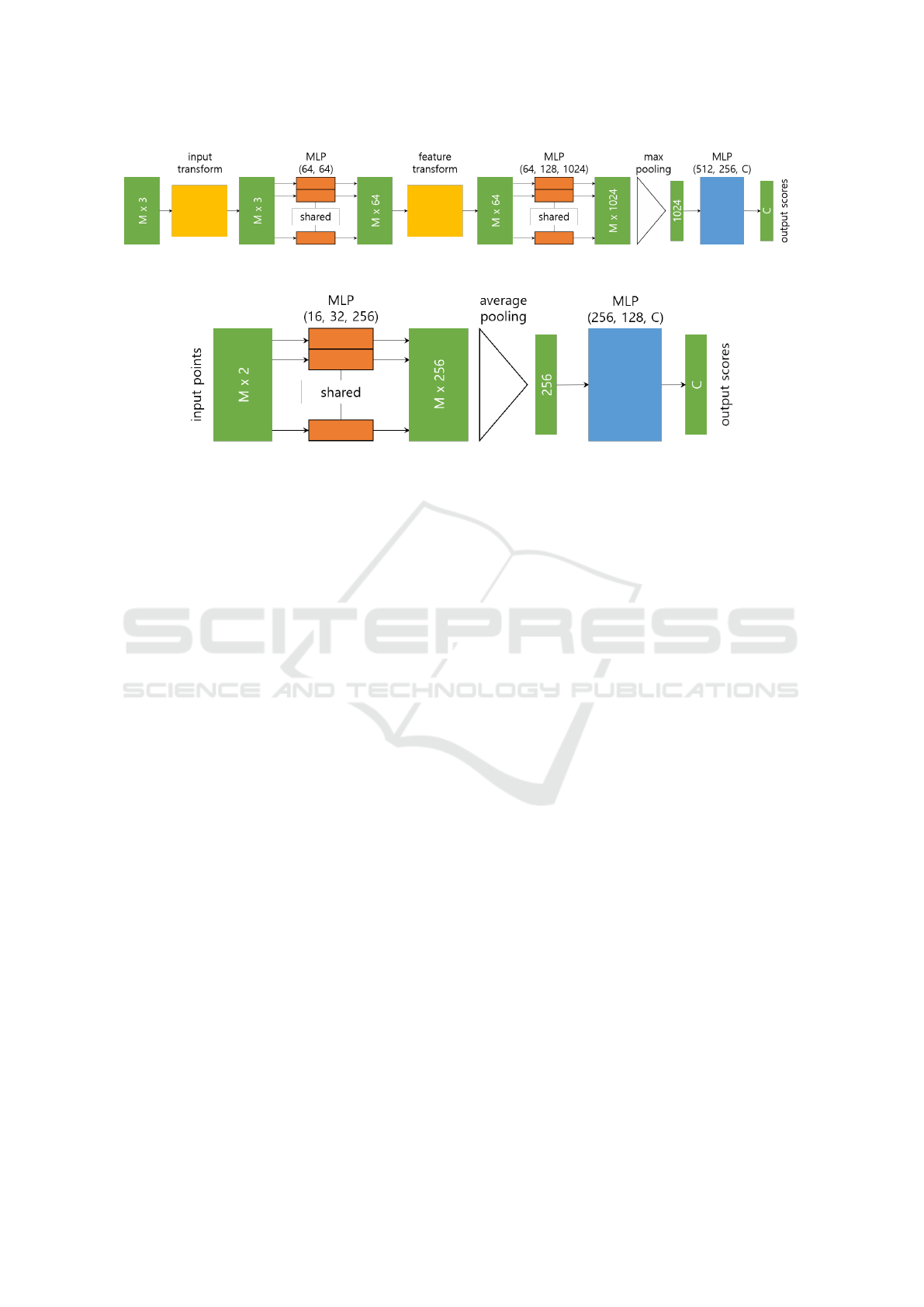
Figure 3: The archtiectures of PointNet and TrajNet. (a) PointNet for point cloud classiﬁcation. (b) TrajNet using average-

pooling layer (TrajNet-A) for vehicle trajectory classiﬁcation. Best viewed in color.

sion and the CNN architecture seem to be simple, it

was veriﬁed in (Santhosh et al., 2018) that it provided

better classiﬁcation performances than other methods

presented for the same purpose.

3 PROPOSED METHOD

According to (Qi et al., 2017), the PointNet archi-

tecture consists of three key modules for point cloud

classiﬁcation and semantic segmentation. Two mod-

ules among them are related to point cloud classiﬁ-

cation, which is similar to the trajectory classiﬁcation

addressed in this work. Associated with the two mod-

ules, we pay attention to the differences between the

properties of trajectory and point cloud. One of the

differences is the fact that the points in a trajectory

are ordered in time sequence different from the points

in a point cloud. The next difference is related to the

fact that the point cloud classiﬁcation should be in-

variant under any rigid transformation, but we do not

have to consider those transformations when classify-

ing a trajectory in this study. Based on the above two

differences, we derive a new network by modifying

the architecture of PointNet. Because of the ﬁrst dif-

ference, we consider using the average-pooling layer

and the ﬂatten layer along with the max-pooling layer.

Note the fact that only the max-pooling layer is used

in the PointNet architecture as shown in Fig. 3a.

Also, PointNet has the joint alignment networks for

the invariance under rigid transformations, which cor-

respond to the blocks denoted as input transform and

feature transform in Fig. 3a. However, the alignment

network is not used in our architecture based on the

second difference.

Based on the two modiﬁcations, we propose the

TrajNet architecture as shown in Fig. 3b. It consists

of three parts, the shared multi-layer perceptrons lay-

ers (MLP), the pooling layers, and the conventional

MLP layers. In the ﬁgure, the average-pooling layer

is used, but it can be replaced by the max-pooling

layer or the ﬂatten layer so that the proposed archi-

tecture is named as TrajNet-M, TrajNet-A, or TrajNet-

F when using the max-pooling, the average pooling,

or the ﬂatten layer, respectively. In detail, the size of

each ﬁlter in the shared MLPs is set to 1, and the num-

bers of those ﬁlters are determined as 16, 32, and 256.

And, we set the dimensions of the two hidden layers

in the conventional MLP to 256 and 128. Each layer

of the shared MLPs and the conventional MLPs em-

ploy the ReLU activation function. The batch normal-

ization (Ioffe and Szegedy, 2015) also follows each

layer of the shared and conventional MLPs. Further-

more, the dropout layer (Srivastava et al., 2014) is

adopted in the two conventional MLPs, and its drop

rate is set to 0.7. Finally, the last layer is the soft-

max for classiﬁcation. The above values of the pa-

rameters were determined from many trials of exper-

iments. Note that the proposed network has a simple

architecture compared to PointNet and the numbers

of the neurons in the MLPs of TrajNet are reduced to

a quarter or a half as shown in Fig 2. It may seem that

the proposed architecture is obtained by only slight

modiﬁcations of the PointNet architecture. However,

it is noticeable that those modiﬁcations are based on

analyzing the differences between trajectory and point

TrajNet: An Efﬁcient and Effective Neural Network for Vehicle Trajectory Classiﬁcation

411

(a) CROSS dataset (b) TRAFFIC dataset (c) VMT dataset

Figure 4: Trajectory examples for three datasets. In the ﬁgures, each cross means the starting point of the trajectory. Best

viewed in color.

Table 1: Datasets used in experiments.

Dataset C N

min

max

CROSS 19 1900 9500 4 30

TRAFFIC 11 300 50 50

VMT 15 1500 16 612

cloud. It will also be veriﬁed in the next section that

the proposed network derived by the simple modiﬁ-

cations is more effective and efﬁcient than the other

networks used in the previous studies for vehicle tra-

jectory classiﬁcation.

4 EXPERIMENTS

We conducted experiments using three datasets

evaluate the neural networks described in the previ-

ous sections. Table 1 summarizes the three datasets

and Fig. 4 shows the examples of trajectories belong-

ing to each class in each dataset. In the table, C, N

and N

denote the number of classes, the number of

training trajectories, and the number of test trajecto-

ries, respectively. Also, M

min

and M

max

denote the

minimum and maximum numbers of points included

in a trajectory in each dataset, respectivley. In Fig. 4,

each trajectory is represented as a curve for better vi-

sualization, but it consists of two-dimensional points

in actual. Among the datasets, the CROSS dataset

(Morris and Trivedi, 2009) has the trajectories gener-

ated by simulating vehicle movements at a four-way

intersection. This dataset provides a training set and

a test set separately. Each trajectory belongs to one

of 19 classes, but its test set contains the trajectories

that do not belong to any class in the training set. Al-

though they can be used for anomaly detection as in

The datasets were downloaded from https:

//github.com/mcximing/ACCV18 Anomaly/tree/master/

Exp2/datasets

(Ma et al., 2018) and (Santhosh et al., 2018), they

were not used in this study to focus on the trajec-

tory classiﬁcation. On the other hand, different from

the CROSS dataset, the TRAFFIC (Lin et al., 2017)

and VMT (Morris and Trivedi, 2011) datasets consist

of the real trajectories extracted by tracking vehicles

captured by a mounted intersection monitoring cam-

era. The TRAFFIC and VMT datasets consist of 11

and 15 classes, respectively, as in Table 1.

Another difference between the CROSS dataset

and the other datasets is the fact that the TRAFFIC

and VMT datasets are not divided as the training set

and test set. In this situation, one of the most general

evaluation methodologies is cross validation. We also

performed the two- and ﬁve-fold cross validations us-

ing the TRAFFIC and VMT datasets, respectively, to

evaluate the performance of the proposed networks.

In K-fold cross validation, the whole trajectories in a

dataset were divided into K folds. The performance

of each network is evaluated using the trajectories in

a fold after training the network using the trajectories

in the other K − 1 folds. These training and testing

procedures are repeated K times utilizing each fold

for testing and the other folds for training at a time.

We ﬁrst compared the neural networks mentioned

in the previous sections in terms of classiﬁcation ac-

curacy. The classiﬁcation accuracy of a network was

computed as

× 100,

where N

is the number of the trajectories that are cor-

rectly classiﬁed among the test trajectories and N is

the number of the whole test trajectories. However,

due to the randomness in weight initialization, the

value of N

may vary even if the same learning is re-

peated. To avoid the problem, we computed the clas-

siﬁcation accuracy whenever the weights of a network

are updated using a mini-batch, and then repeated the

same training and evaluation ten times for a given pair

of the training and test sets. We selected the maxi-

mum value of N

to compute the classiﬁcation accu-

ICPRAM 2021 - 10th International Conference on Pattern Recognition Applications and Methods

412

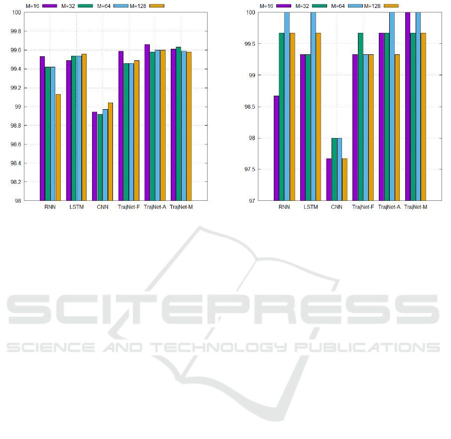
Figure 5: Classiﬁcation results for CROSS dataset. Best

viewed in color.

racy in those repetitive training and testing. In the

K-cross validation, the maximum number of the cor-

rectly classiﬁed trajectories was selected for each pair

of training and test sets, and the value of N

was de-

termined by adding the K maximum numbers for all

of the pairs of the training and test sets.

We implemented all of the methods described in

this section using TensorFlow (Abadi et al., 2015).

The cross entropy was chosen as the loss function in

training all of the networks, and we adopted the Adam

optimizer (Kingma and Ba, 2015) with the learning

rate of 0.001 to minimize (maximize) the loss func-

tion. The size of the mini-batch was set to 100 when

training all of the networks. From many trials of those

network training, the maximum number of epochs

was set to 500, 500, 50, and 400 for RNN, LSTM,

CNN, and TrajNets, respectively. This means that

CNN could be easily trained compared to the other

networks. To examine the relationship between the

number of points in trajectories and the classiﬁcation

performance, we performed the experiments by vary-

ing the value of M as 16, 32, 64, and 128.

Figures 5, 6, and 7 show the classiﬁcation ac-

curacies for the CROSS, TRAFFIC, VMT datasets,

respectively. It is shown in Fig. 5 that all of the

networks provided classiﬁcation accuracies over 99%

on average except for CNN, which showed its aver-

age accuracy of 98.97% for the CROSS dataset. In

particular, TrajNet-A and TrajNet-M, which are the

proposed networks, yielded the best average perfor-

mances over 99.6%, and TrajNet-A obtained the high-

est classiﬁcation accuracy with M = 16. We can see

that RNN yielded lower classiﬁcation accuracies as

Figure 6: Classiﬁcation results for TRAFFIC dataset. Best

viewed in color.

M increases. This agrees with the fact well-known

in the literature that the learning capability of RNN

decreases when the length of the sequence data in-

creases. However, the proposed networks can provide

slightly higher accuracies with the small numbers of

M than RNN, LSTM, and CNN. Since the time re-

quired for the inference of an arbitrary trajectory in-

creases with the value of M, this means that the pro-

posed network can classify trajectories in a shorter

time. Figure 6 shows the classiﬁcation accuracies of

the networks on the TRAFFIC dataset. Similar to the

CROSS dataset, we can see that CNN provided the

lowest classiﬁcation accuracies for all the values of

M. Note that the 100% classiﬁcation accuracy was

obtained by RNN, LSTM, TrajNet-A, and TrajNet-

M when M = 64. However, TrajNet-A and TrajNet-

M yielded the highest average accuracies of 99.67%

and 99.84%, respectively, and TrajNet-M provided

100% accuracy when M = 16 as well as M = 64. Fig-

ure 7 shows the classiﬁcation accuracies on the VMT

dataset. We can see again that the accuracy of RNN

decreases relatively large as the value of M increases.

On average, TrajNet-A, TrajNet-M, and LSTM pro-

vided the highest accuracies of 99.10%, 99.02%, and

99.00%, respectively. It is notable that TrajNet-A

provided the best accuracies for M = 16, M = 32,

and M = 128. In particular, the highest accuracy

of 99.2% on this dataset was obtained by TrajNet-A

when M = 16. In total, it may seem that the accuracy

improvement of the proposed networks is marginal.

However, the improvements are not meaningless be-

cause RNN, LSTM, and CNN already give very high

accuracies of around 99%.

TrajNet: An Efﬁcient and Effective Neural Network for Vehicle Trajectory Classiﬁcation

413

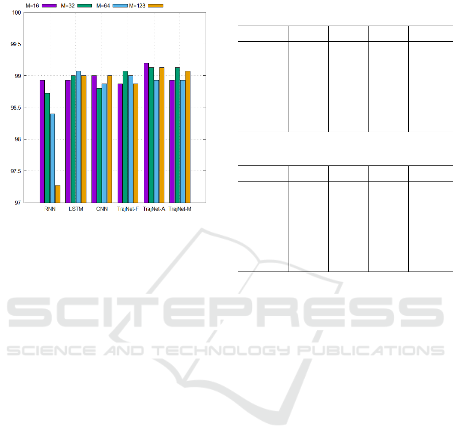
Figure 7: Classiﬁcation results for VMT dataset. Best

viewed in color.

Together with the classiﬁcation accuracy, the clas-

siﬁcation speed and the number of parameters are also

important performance of classiﬁcation methods. We

measured the inference time required to classify tra-

jectories and counted the number of parameters in the

networks. Table 2 shows the time to classify the 9500

test trajectories in the CROSS dataset after training

each network for all the values of M. It was mea-

sured on a PC with a GPU of TITAN Xp. In the

case of CNN, the time required in the conversion from

an input trajectory to an image was not included in

the inference time. The table shows that the pro-

posed networks can classify input trajectories faster

than RNN, LSTM, and CNN for each value of M.

In particular, when M = 16, TrajNet-A, which gave

better classiﬁcation accuracies, required about 40%,

59%, and 45% of the inference times of RNN, LSTM,

and CNN, respectively. Note that those speed im-

provements were achieved together with the improve-

ment in the classiﬁcation accuracy, not its sacriﬁce.

As M increases, we can see that the inference time

increases in all of the networks except CNN. How-

ever, the ones of TrajNets increase slower than the

ones of RNN and LSTM. It can be expected from

this result that the trajectory classiﬁcation based on

TrajNet can be performed much faster than RNN or

LSTM in a situation that the points included in trajec-

tories become more and more. Interestingly, TrajNet-

F showed the fastest inference time even though it

contains the maximum number of parameters for the

same value of M. We expect from this result that the

architecture of TrajNet-F is more appropriate to the

use of GPU than the other architectures. Another su-

Table 2: Inference time required to classify 9500 test trajec-

tories in CROSS dataset (in seconds).

Network M = 16 M = 32 M = 64 M = 128

RNN 2.142 3.687 7.661 15.941

LSTM 1.466 1.713 2.126 2.855

CNN 1.926 1.919 1.923 1.921

TrajNet-F

0.549 0.600 0.615 0.714

TrajNet-A 0.865 0.882 0.971 1.097

TrajNet-M 0.930 0.954 1.017 1.143

Table 3: Number of parameters in network (in thousands).

Network M = 16 M = 32 M = 64 M = 128

RNN 102 102 102 102

LSTM 351 351 351 351

CNN 189 189 189 189

TrajNet-F 1095 2145 4241 8436

TrajNet-A 113 113 113 113

TrajNet-M 113 113 113 113

periority of the proposed networks can be seen in Ta-

ble 3, which summarizes the number of parameters

for each value of M. We can see from the table that re-

gardless of the value of M, the numbers of parameters

included in all of the networks remain the same except

TrajNet-F. Among those networks, the two proposed

networks, TrajNet-A and TrajNet-M, contain the low-

est numbers of parameters except for RNN.

In summary, it was demonstrated from our exper-

imental results on the three datasets that TrajNet can

classify an input trajectory faster and more accurately

than the other deep networks presented in the previ-

ous studies, and the proposed architecture with the

average-pooling or the max-pooling layer can also be

stored in a less memory space than LSTM and CNN.

5 CONCLUSIONS

In this paper, we proposed a new network architecture

to address the vehicle trajectory classiﬁcation. In-

spired from PointNet (Qi et al., 2017), which has a

novel architecture to deal with point cloud classiﬁca-

tion and semantic segmentation, the proposed archi-

tecture was derived based on analyzing the difference

between the properties of the trajectory and the point

cloud. From our experiments using the three public

datasets, we show that the proposed architecture could

provide slight improvements in the classiﬁcation ac-

curacy over RNN, LSTM, and CNN, which yielded

ICPRAM 2021 - 10th International Conference on Pattern Recognition Applications and Methods

414

sufﬁciently high classiﬁcation accuracies. Further-

more, it was veriﬁed that TrajNet-A, one of the pro-

posed networks, could classify the test trajectories of

the CROSS dataset in 40%, 59%, and 45% less time

than RNN, LSTM, and CNN, respectively, under the

setting of M = 16 along with the accuracy improve-

ments. In terms of memory space, TrajNet-A and

TrajNet-M require lower numbers of parameters than

LSTM and CNN. Also, we could see from the exper-

iments that the number of points included in a tra-

jectory has little effect on the classiﬁcation accuracy

except for RNN.

In future work, the proposed networks will be ap-

plied in classifying the vehicle trajectories extracted

from various real trafﬁc situations with trajectory gen-

eration methods for trafﬁc ﬂow measurement and

anomaly detection at intersections. Moreover, we ex-

pect that the proposed networks can be utilized in

classifying trajectories obtained in other applications

such as online handwriting recognition (Kim and Sin,

2014) and human activity recognition (Anguita et al.,

2013).

ACKNOWLEDGEMENTS

This work was supported by Electronics and Tele-

communications Research Institute (ETRI) grant

funded by the Korean government [20ZD1110, De-

velopment of ICT Convergence Technology for

Daegu-Gyeongbuk Regional Industry].

REFERENCES

Abadi, M., Agarwal, A., Barham, P., Brevdo, E., Chen, Z.,

Citro, C., Corrado, G. S., Davis, A., Dean, J., Devin,

M., Ghemawat, S., Goodfellow, I., Harp, A., Irving,

G., Isard, M., Jia, Y., Jozefowicz, R., Kaiser, L., Kud-

lur, M., Levenberg, J., Man

e, D., Monga, R., Moore,

S., Murray, D., Olah, C., Schuster, M., Shlens, J.,

Steiner, B., Sutskever, I., Talwar, K., Tucker, P., Van-

houcke, V., Vasudevan, V., Vi

egas, F., Vinyals, O.,

Warden, P., Wattenberg, M., Wicke, M., Yu, Y., and

Zheng, X. (2015). TensorFlow: Large-Scale Machine

Learning on Heterogeneous Systems. Software avail-

able from tensorﬂow.org.

Anguita, D., Ghio, A., Oneta, L., Parra Perez, X., and Reyes

Ortiz, J. L. (2013). A public domain dataset for human

activity recognition using smartphones. In Proceed-

ings of the 21th International European Symposium

on Artiﬁcial Neural Networks, Computational Intelli-

gence and Machine Learning, pages 437–442.

Goodfellow, I., Bengio, Y., and Courville, A. (2016). Deep

Learning. The MIT Press.

Hu, W., Li, X., Tian, G., Maybank, S., and Zhang, Z.

(2013). An Incremental DPMM-Based Method for

Trajectory Clustering, Modeling, and Retrieval. IEEE

Transactions on Pattern Analysis and Machine Intel-

ligence, 35(5):1051–1065.

Ioffe, S. and Szegedy, C. (2015). Batch Normalization: Ac-

celerating Deep Network Training by Reducing Inter-

nal Covariate Shift. In ICML’15: Proceedings of the

32nd International Conference on International Con-

ference on Machine Learning, volume 37, pages 448–

456.

Jiang, X., de Souza, E. N., Pesaranghader, A., Hu, B.,

Silver, D. L., and Matwin, S. (2017). Trajecto-

ryNet: An Embedded GPS Trajectory Representation

for Point-based Classiﬁcation Using Recurrent Neural

Networks. In Proceedings of the 27th Annual Interna-

tional Conference on Computer Science and Software

Engineering, pages 192–200.

Kim, J. and Sin, B.-K. (2014). Online Handwriting Recog-

nition. In Doermann, D. and Tombre, K., editors,

Handbook of Document Image Processing and Recog-

nition, pages 887–915. Springer London, London.

Kingma, D. and Ba, J. (2015). Adam: A Method for

Stochastic Optimization. International Conference on

Learning Representations (ICLR).

Krizhevsky, A., Sutskever, I., and Hinton, G. E. (2012). Im-

ageNet Classiﬁcation with Deep Convolutional Neu-

ral Networks. In Advances in Neural Information Pro-

cessing Systems 25, pages 1097–1105.

Li, X., Chen, M., Nie, F., and Wang, Q. (2017).

A Multiview-Based Parameter Free Framework for

Group Detection. In Proceedings of the Thirty-First

AAAI Conference on Artiﬁcial Intelligence, pages

4147–4153. AAAI Press.

Lin, W., Zhou, Y., Xu, H., Yan, J., Xu, M., Wu, J., and

Liu, Z. (2017). A Tube-and-Droplet-Based Approach

for Representing and Analyzing Motion Trajectories.

IEEE Transactions on Pattern Analysis and Machine

Intelligence, 39(8):1489–1503.

Lv, Y., Duan, Y., Kang, W., Li, Z., and Wang, F. (2015).

Trafﬁc Flow Prediction With Big Data: A Deep

Learning Approach. IEEE Transactions on Intelligent

Transportation Systems, 16(2):865–873.

Ma, C., Miao, Z., Li, M., Song, S., and Yang, M.-H. (2018).

Detecting Anomalous Trajectories via Recurrent Neu-

ral Networks. In Jawahar, C., Li, H., Mori, G., and

Schindler, K., editors, Computer Vision – ACCV 2018,

pages 370–382, Cham. Springer International Pub-

lishing.

Morris, B. T. and Trivedi, M. (2009). Learning Trajec-

tory Patterns by Clustering: Experimental Studies and

Comparative Evaluation. In 2009 IEEE Conference

on Computer Vision and Pattern Recognition, pages

312–319.

Morris, B. T. and Trivedi, M. M. (2011). Trajectory Learn-

ing for Activity Understanding: Unsupervised, Mul-

tilevel, and Long-Term Adaptive Approach. IEEE

Transactions on Pattern Analysis and Machine Intel-

ligence, 33(11):2287–2301.

TrajNet: An Efﬁcient and Effective Neural Network for Vehicle Trajectory Classiﬁcation

415

Nair, V. and Hinton, G. E. (2010). Rectiﬁed Linear Units

Improve Restricted Boltzmann Machines. In Proceed-

ings of the 27th International Conference on Machine

Learning, pages 807–814. Omnipress.

Porikli, F. (2004). Trajectory Distance Metric Using Hid-

den Markov Model based Representation. In Sixth

IEEE International Workshop on Performance Eval-

uation of Tracking and Surveillance.

Qi, C. R., Su, H., Mo, K., and Guibas, L. J. (2017). Point-

Net: Deep Learning on Point Sets for 3D Classiﬁ-

cation and Segmentation. In 2017 IEEE Conference

on Computer Vision and Pattern Recognition (CVPR),

pages 77–85.

Ren, S., He, K., Girshick, R., and Sun, J. (2015). Faster R-

CNN: Towards Real-Time Object Detection with Re-

gion Proposal Networks. In Advances in Neural Infor-

mation Processing Systems 28, pages 91–99.

Ren, X., Wang, D., Laskey, M., and Goldberg, K. (2018).

Learning Trafﬁc Behaviors by Extracting Vehicle Tra-

jectories from Online Video Streams. In 2018 IEEE

14th International Conference on Automation Science

and Engineering (CASE), pages 1276–1283.

Santhosh, K. K., Dogra, D. P., Roy, P. P., and Mi-

tra, A. (2018). Video Trajectory Classiﬁcation and

Anomaly Detection Using Hybrid CNN-VAE. CoRR,

abs/1812.07203.

Song, L., Wang, R., Xiao, D., Han, X., Cai, Y., and Shi, C.

(2018). Anomalous Trajectory Detection Using Re-

current Neural Network. In Gan, G., Li, B., Li, X., and

Wang, S., editors, Advanced Data Mining and Appli-

cations, pages 263–277, Cham. Springer International

Publishing.

Srivastava, N., Hinton, G., Krizhevsky, A., Sutskever, I.,

and Salakhutdinov, R. (2014). Dropout: A Simple

Way to Prevent Neural Networks from Overﬁtting.

Journal of Machine Learning Research, 15:1929–

1958.

Wang, J. M., Fleet, D. J., and Hertzmann, A. (2008). Gaus-

sian Process Dynamical Models for Human Motion.

IEEE Transactions on Pattern Analysis and Machine

Intelligence, 30(2):283–298.

Wang, X., Ma, K. T., Ng, G.-W., and Grimson, W. L.

(2011). Trajectory Analysis and Semantic Re-

gion Modeling Using Nonparametric Hierarchical

Bayesian Models. International Journal of Computer

Vision, 95:287–312.

Xu, H., Zhou, Y., Lin, W., and Zha, H. (2015). Un-

supervised Trajectory Clustering via Adaptive Multi-

kernel-Based Shrinkage. In 2015 IEEE International

Conference on Computer Vision (ICCV), pages 4328–

4336.

Yang, J. B., Nguyen, M. N., San, P. P., Li, X. L., and Kr-

ishnaswamy, S. (2015). Deep Convolutional Neural

Networks on Multichannel Time Series for Human

Activity Recognition. In Proceedings of the Twenty-

Fourth International Joint Conference on Artiﬁcial In-

telligence (IJCAI), pages 3995–4001.

Yao, D., Zhang, C., Zhu, Z., Huang, J., and Bi, J. (2017).

Trajectory clustering via deep representation learning.

In 2017 International Joint Conference on Neural Net-

works (IJCNN), pages 3880–3887.

Zhao, J., Yi, Z., Pan, S., Zhao, Y., Zhao, Z., Su, F., and

Zhuang, B. (2019). Unsupervised Trafﬁc Anomaly

Detection Using Trajectories. In The IEEE Confer-

ence on Computer Vision and Pattern Recognition

(CVPR) Workshops.

ICPRAM 2021 - 10th International Conference on Pattern Recognition Applications and Methods

416