
Decentralized Multi-agent Formation Control via Deep
Reinforcement Learning
Aniket Gutpa
1,*
and Raghava Nallanthighal
2,†
1
Department of Electrical Engineering, Delhi Technological University, New Delhi, India
2
Department of Electronics and Communication Engineering, Delhi Technological University, New Delhi, India
Keywords: Multi-agent Systems, Swarm Robotics, Formation Control, Policy Gradient Methods.
Abstract: Multi-agent formation control has been a much-researched topic and while several methods from control
theory exist, they require astute expertise to tune properly which is highly resource-intensive and often fails
to adapt properly to slight changes in the environment. This paper presents an end-to-end decentralized
approach towards multi-agent formation control with the information available from onboard sensors by using
a Deep Reinforcement learning framework. The proposed method directly utilizes the raw sensor readings to
calculate the agent’s movement velocity using a Deep Neural Network. The approach utilizes Policy gradient
methods to generalize efficiently on various simulation scenarios and is trained over a large number of agents.
We validate the performance of the learned policy using numerous simulated scenarios and a comprehensive
evaluation. Finally, the performance of the learned policy is demonstrated in new scenarios with non-
cooperative agents that were not introduced during the training process.
1 INTRODUCTION
Multi-agent systems are rapidly gaining momentum
due to their several real-world applications in disaster
relief scenarios, rescue operations, military
operations, warehouse management, agriculture and
many more. All these tasks require the teams of
robots to cooperate autonomously to produce the
desired results as displayed by many animals and
insects in nature which emulate swarming behaviour.
One of the major challenges for multi-agent
systems is autonomous navigation while adhering to
the three rules of Reynolds (Reynolds and Craig,
1987). Modern control theory presents numerous
solutions, supported with rigorous proofs, to this
problem and demonstrates the feasibility of multi-
agent formation control and obstacle avoidance.
(Marko and Stiepan, 2012), (Anuj et al., 2020),
(Egerestedt, 2007) present an artificial potential field
approach and have demonstrated stable autonomous
navigation of a swarm of unmanned aerial vehicles
(UAVs). While this approach does the work, it
neglects the non-linearities in the system dynamics
and thus fails to demonstrate optimal behaviour in
*
http://www.dtu.ac.in/Web/Departments/Electrical/about/
†
http://www.dtu.ac.in/Web/Departments/Electronics/about/
conjunction with the vehicle dynamics. Further, these
approaches require extensive tuning to provide
desired performance.
Further, in (Hung and Givigi, 2017), a Q-learning
based controller is presented for flocking of a swarm
of UAVs in unknown environments using a leader-
follower approach. This approach does not yield an
optimal solution as state space and action space is
discretized to limit the size of the Q-table. As the
number of states increases, computing the Q-table
becomes increasingly inefficient. Another
disadvantage of this approach is the single point of
failure offered by the leader agent.
In (Johns and Rasmus, 2018), Reinforcement
learning is utilized to improve the performance of a
behaviour-based control algorithm which serves as
both a baseline from which the RL algorithm
compares with and a base from which the RL
algorithm starts training. This approach produces
significant results but is not an end to end solution
which can be directly applied to any kind of system.
Appropriate tuning of the behaviour-based control
algorithm is still required for the efficient
performance of the complete controller.
Gutpa, A. and Nallanthighal, R.
Decentralized Multi-agent Formation Control via Deep Reinforcement Learning.
DOI: 10.5220/0010241302890295
In Proceedings of the 13th International Conference on Agents and Artificial Intelligence (ICAART 2021) - Volume 1, pages 289-295
ISBN: 978-989-758-484-8
Copyright
c
2021 by SCITEPRESS – Science and Technology Publications, Lda. All rights reserved
289

The contribution of this paper is to propose a
decentralized, end-to-end framework that is scalable,
adaptive, and fault-tolerant which directly maps the
sensor data to optimal steering commands. To
overcome the problems offered by discrete state space
and discrete action space controllers, we propose a
policy gradient-based controller, which utilizes a
Deep neural network map the continuous state space
directly to a continuous action space. The
effectiveness of policy learned from the proposed
method is demonstrated through a series of simulation
experiments where it is able to find the optimal
trajectories in complex environments.
The rest of the paper is organised as follows:
Section II gives a short introduction to Policy
Gradient methods and leads on for the mathematical
formulation of our problem statement in the context
of RL. Section III introduces the proposed algorithm
and the underlying structure of the complete
controller for decentralized implementation.
Subsequently, section IV describes the simulation
environment, the computational complexity of our
approach and presents the quantitative results
obtained. Further, it also provides the experimental
results in unknown environments to demonstrate the
generalization capability of the learned policy.
Finally, Section V concludes the paper with
recommendations for future work.
2 PRELIMINARIES
2.1 Markov Decision Process
A Markov decision process (Bellman and Richard,
1957) is a finite transition graph which satisfies the
markov property. For a single agent MDP can be
represented by a tuple ,, where
,…,
is the set of states,
,…,
is
the set of actions and
,…,
is the set of
rewards obtained by through transition between states
(
represents the terminal state). The objective is to
find the solution of this MDP to maximize the
expected sum of rewards by finding the optimal
policy, value function or action-value function.
2.2 Deep Q-learning
Deep Q-learning (Mnih et al., 2015) is one of the
well-known methods in Deep RL and has been shown
to provide extremely efficient results. It uses deep
neural networks for estimating the action-value
function for a given problem to identify the optimal
action in any state. The estimator function can be
described as:
,
~
,
max
,
(1)
where, is the denotes the expectation operator.
Therefore, if the neural network representing the Q
function is given by parameters , the loss function
can be given by:
,
,,,
~
,
(2)
1
max
,
is called the
temporal difference and is calculated using target
network Q^π' which is updated with the same
parameters as main Q-function periodically. This
method stores the set of experiences generated over
time into the Replay buffer which is used to randomly
sample data for training the loss function given above.
2.3 Policy Gradient Algorithms
Policy gradient algorithms explicitly denote the
policy as
| represented by a deep neural
network with parameter . These parameters can be
trained by maximizing the objective function
~,~
, where R is the reward
function. Thus, to update the policy parameters,
gradient ascent can be used by calculating the
gradient of the objective function.
|
(3)
Where,
~,~
log
|
These methods can be used for both stochastic as
well as deterministic policies and thus are suitable for
problems with continuous action spaces.
2.4 Algebraic Graph Theory
A complete multi-agent system can be
mathematically represented by a weighted undirected
graph
,
where1,2,…, is the set of
agents and
,
:,∈,is the edge set.
The adjacency matrix of graph represented by
is a standard matrix in graph theory which
represents the weights of the edges. This matrix can
be used to represent the relationship between agents.
ICAART 2021 - 13th International Conference on Agents and Artificial Intelligence
290

3 PROBLEM FORMULATION
In this paper, the task of formation flocking is defined
in the context of holonomic agents moving on the
Euclidean plane. The position vector for each agent
can be denoted by
,
and the velocity
vector by
,
, for the UAV i (i = 1, 2, …,
N) at time t, where N is the number of UAVs. The
goal of the agents is to attain the desired formation
using the adjacency matric
of the formation
matrix graph
(where the weight of each edge
, of the graph corresponds to the desired distance
between the agents and ) and navigate to the goal
position
,
while avoiding inter-agent
collisions. To maintain the formation at the goal
position, another adjacency matrix
of graph
(where the weight of each edge ,
of the
graph corresponds to the desired distance between the
agent and goal position
.
Thus, the problem statement can be modelled as a
sequential MDP defined by a tuple ,,,
where,
,…
,
,…,
,
,…,
,
,…,
is the set of sets of
states, actions, rewards and observations of all agents.
At time step t, agent is present in state and has
access to an observation o, which is used to calculate
action . As a consequence of this action, the agent
reaches a new state ′, receives a reward and has
access to new observation ′. The goal of the agent is
to learn the optimal policy
∗
| where denotes
the policy parameters which maximizes the sum of
obtained rewards. This process continues until all the
agents reach the goal position where the episode
terminates.
The sequence of the tuple ,,,′ made by the
robot can be considered as a trajectory denoted by
. The set of these trajectories collected by all the
agents is denoted by and is stored in memory as the
Replay buffer. denotes the minibatch of
experiences randomly samples from for training
the model.
4 APPROACH
4.1 Environmental Setup
To solve the sequential MDP defined in Section III,
an environmental model with appropriately defined
observation space, action space and reward function
is required.
4.1.1 Observation Space
The observation space o consists of the planar
position of each agent given by
along with the goal
position
. These values are flattened and passed to
a fully connected input layer of the policy network to
calculate the action values. Thus, the size of input
layer varies with the number of agents which also
increases the training time for the policy network.
4.1.2 Action Space
The holonomic agents considered for the problem
statement have an action space that consists of a set
of permissible velocities in the continuous space. The
output action is the two-dimensional velocity vector
,
. The output layer is constrained by the
hyperbolic tangent activation function which
limits the output value in the range of (-1,1). This
output value is then multiplied by
parameter to
limit the action value, which is then directly passed to
the navigation controller of the agent.
4.1.3 Reward Function
To achieve the target of formation control and
navigation in the minimum time possible, the reward
function is designed as follows:
(4)
where, the total reward
is the sum of goal
reward
, formation reward
and inter-agent
collision penalty
of an agent at timestep .
The goal reward
is awarded for the agent
for reaching the goal position as:
,
,
,
,
(5)
To maintain the desired formation as governed by
the formation graph
, the agents are penalized for
deviating from their desired relative position with
other agents as:
,
,
(6)
Finally, to avoid inter-agent collisions, the agents
are penalized as follows:
,
0,
,
(7)
Decentralized Multi-agent Formation Control via Deep Reinforcement Learning
291
Algorithm 1: Multi-agent TD3.
1:
I
nitialize policy network with parameters , Q-
f
unctions with parameters
,
. Empty the repla
y
b
uffer
2: Set target network parameters equal to mai
n
p
arameters
←,
,
←
,
,
←
3:
f
or number of episodes do
4:
for robot 1,2,… do
5:
Take observation
select action
,
,
6:
Execute action in the environment
7:
Observe next state ′, reward and done signa
l
to indicate whether o′ is terminal.
8:
Store ,,,′, in replay buffer
9:
If ′ is terminal, reset environment state.
10:
end for
11: if memory can provide minibatch then
12: Randomly sample a batch of transitions,
,,,′,
from
13: Compute target actions
,
,
,,
14: Compute Bellman target
,
,
1
min
,
,
,
15: Update Q-functions by one step of gradien
t
d
escent using
1
|
|
,
,
,
,,
,
∈
1,2
16: if time to update policy then
17: Update policy by one step of gradient ascen
t
u
sing
1
|
|
,
∈
18: Update target networks with
←
1
,
←
,
1
1,2
19:
end if
20:
end if
21:
end for
4.2 Algorithm Design
The algorithm used in this paper is an extended
version of the state-of-the-art Twin Delayed
Deterministic Policy Gradient algorithm (Fujimoto et
al., 2018), (Lillicrap et al., 2015)) commonly known
as TD3. TD3 concurrently learns two Q-functions and
a policy and uses the smaller out of the two Q-values
to calculate the loss function. We use the paradigm of
centralized training with decentralized execution,
which means that the data collected by all the agents
is used for training the policy network
|, but
each agent takes action in a decentralized fashion by
using this policy.
During each episode of the training process, there
are two major steps. First, all the agents exploit the
same policy to calculate their actions and record their
new observations which are then stored in the replay
buffer. Second, random batches of experiences are
sampled from the replay buffer to calculate the
Bellman target which is used to calculate the loss
function as given in eq.2. This loss is optimized using
Adam optimizer (Kingma et al., 2014). Further, for
policy training, the problem statement requires a
deterministic policy
|
which gives the action
that maximizes the Q-function. Therefore, the
objective function can be modified as
max
~
,
(8)
and therefore, the policy gradient can be calculated as
1
|
|
,
∈
(9)
The target networks in the algorithm are updated
periodically using the Polyak averaging method as
follows:
←
1
(10)
,
←
,
1
;1,2
(11)
where ≪1.
4.3 Network Architecture
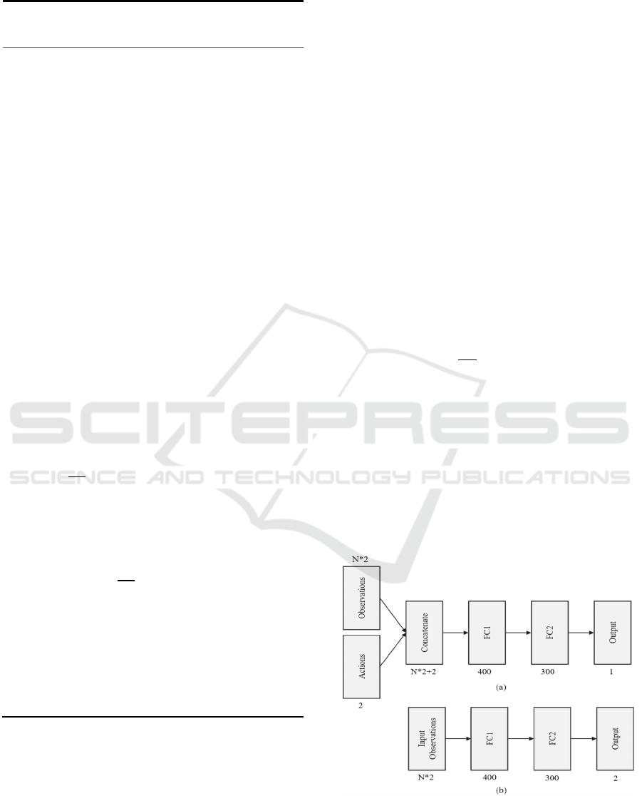
Figure 1: Network architecture of the (a) critic and (b) actor
neural networks.
ICAART 2021 - 13th International Conference on Agents and Artificial Intelligence
292
TD3 algorithm utilizes six neural networks in total,
three main and three target networks. The target
networks are employed to stabilize the training
process. The observation o with dimensions
∗2∗
1
directly acts as the input for the policy network and
outputs the action value. While for the Q-network,
observation o and action a are concatenated to form
the input layer and the output is a single Q-value
which gives the quality of that action. The network
architecture for both policy network and the Q-
network is given in Figure.1. RELU activation
function is used for the hidden layers while the output
layer utilizes a ‘tan h’ activation function to limit the
output velocity by a maximum limit.
5 SIMULATION AND TESTING
In this section, first the method of simulation is
explained. Then, the computational complexity of the
algorithm and training resources utilized is described.
Lastly, the quantitative results of various simulations
in varying environments are demonstrated.
5.1 Simulation Environment
The simulation environment is a custom developed
GUI using Matplotlib library in python. The blue
circles represent the agents, the red circle is the goal
and the black circles are the obstacles.
The start position of the agents, goal position and
all the obstacles are randomly generated after each
episode is over. This approach was found to prevent
the policy from exploiting the errors in the Q-function
and thus improved the performance of the algorithm
substantially.
5.2 Training Configuration
The complete implementation was carried out using
TensorFlow 2 on a computer with a Nvidia GTX 1060
GPU and an Intel i7-8750 CPU with the set of hyper-
parameters as mentioned in Table 1. The complete
training process took about 22 hours for the learned
policy to achieve robust performance in a complete
simulation of 10 agents.
During the execution, since only the actor network
is required, the computational resources required are
minimal and thus the same architecture can be used
on single-board computers like the Nvidia Jetson
nano and Raspberry Pi.
Table 1: Hyperparameters used for simulation.
Hyperparameter Value
1000
0.99
0.0001
0.001
0.995
1000000
-2
2
Hyperparameter Value
0.1
0.5
10
-50
0.5
1
-0.1
-0.1
5.3 Experiments and Results
Since, the observation space consists of the planar
positions of all the agents and the goal position, the
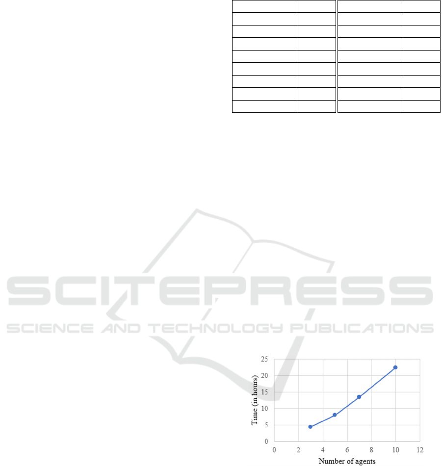
training time increases rapidly as the number of
agents scale up. Figure 3 shows the training time
required for training the policy on three, five, seven
and ten agents respectively.
Further, Figure 3 shows the average reward
received as training progresses. Figure 4-6 shows the
performance of the learned policy on a varying
number of agents for different formations.
To test the generalization capabilities of the
learned policy, we introduced non-cooperative agents
[agents travelling directly towards the goal position in
a straight line with constant velocity] which were not
used during the entire training process. But the
learned policy was able to generalize well with these
agents as demonstrated in Figure 7. (Non-cooperative
agents are shown by square boxes)
Figure 2: Increase in training time with increment in
number of agents.
Decentralized Multi-agent Formation Control via Deep Reinforcement Learning
293
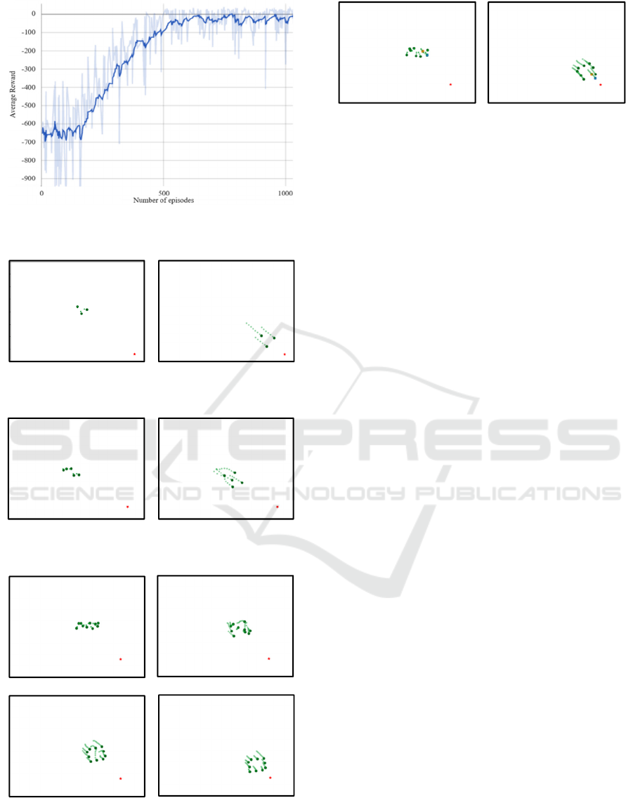
Figure 3: Average rewards progression with increasing
episodes during training process.
(a)
(b)
Figure 4: V-formation using 3 agents.
(a)
(b)
Figure 5: X-formation using 5 agents.
(a)
(b)
(c)
(d)
Figure 6: Diamond-formation using 10 agents.
(a) (b)
Figure 7: Diamond-formation using 8 cooperative and 2
non-cooperative agents.
6 CONCLUSIONS
In this paper, we addressed the problem of Multi-
agent formation control and navigation in unknown
environments by using an end-to-end Deep
Reinforcement Learning framework. The learned
policy demonstrates several advantages over the
existing methods in terms of maintaining the desired
formation, collision avoidance performance,
adaptability to the environments and generalized
performance.
Multi-agent systems are the future of the robotics
industry and as they become more prevalent, these
systems will require adaptive controllers which can
execute the tasks effectively in unfamiliar situations.
Thus, integration of Reinforcement Learning with
multi-agent systems is a step towards developing
truly intelligent systems which can perform
efficiently in real-world. We hope that our work can
serve as the starting step in developing swarming
systems for future applications.
Our future work in this area will be aimed towards
following two goals:
1. Developing an efficient approach to solve the
problem of extended training time with increase in
number of agents.
2. Applying DRL to mission-specific problems
such as target search and area coverage and to apply
better exploration techniques to improve the learning
time of the policy.
REFERENCES
Reynolds, Craig, 1987. Flocks, herds and schools: A
distributed behavioural model. SIGGRAPH '87:
Proceedings of the 14th Annual Conference on
Computer Graphics and Interactive Techniques.
Association for Computing Machinery. pp. 25–34.
Marko Bunic, Stjepan Bogdan, 2012. Potential Function
Based Multi-Agent Formation Control in 3D Space,
IFAC Proceedings Volumes, Volume 45, Issue 22,
Pages 682-689.
ICAART 2021 - 13th International Conference on Agents and Artificial Intelligence
294

Anuj Agrawal, Aniket Gupta, Joyraj Bhowmick, Anurag
Singh, Raghava Nallanthighal, 2020. “A Novel
Controller of Multi-Agent System Navigation and
Obstacle Avoidance”, Procedia Computer Science,
Volume 171, Pages 1221-1230.
M. Egerestedt, 2007. “Graph-theoretic methods for multi-
agent coordination” in ROBOMAT.
S. Hung and S. N. Givigi, 2017. "A Q-Learning Approach
to Flocking with UAVs in a Stochastic Environment,"
in IEEE Transactions on Cybernetics, vol. 47, no. 1, pp.
186-197.
Johns, Rasmus, 2018. “Intelligent Formation Control using
Deep Reinforcement Learning.”.
Mnih, V., Kavukcuoglu, K., Silver, D. et al, 2015. Human-
level control through deep reinforcement learning.
Nature 518, 529–533.
Fujimoto, Scott & Hoof, Herke & Meger, Dave, 2018.
Addressing Function Approximation Error in Actor-
Critic Methods.
Lillicrap, Timothy & Hunt, Jonathan & Pritzel, Alexander
& Heess, Nicolas & Erez, Tom & Tassa, Yuval &
Silver, David & Wierstra, Daan, 2015. Continuous
control with deep reinforcement learning. CoRR.
Kingma, Diederik and Ba, Jimmy, 2014. “Adam: A method
for Stochastic Optimization.”
Bellman, Richard, 1957. “A Markovian Decision
Process.” Journal of Mathematics and Mechanics, vol. 6,
no. 5, pp. 679–684., www.jstor.org/stable/24900506.
Decentralized Multi-agent Formation Control via Deep Reinforcement Learning
295
