Discrete and Continuous Deep Residual Learning over Graphs

Pedro H. C. Avelar

1 a

, Anderson R. Tavares

1 b

, Marco Gori

2 c

and Lu

ıs C. Lamb

1 d

Institute of Informatics, Federal University of Rio Grande do Sul - UFRGS, Porto Alegre, Brazil

Department of Computing, University of Siena, Siena, Italy

Keywords:

Graph Neural Networks, Residual Learning.

Abstract:

We propose the use of continuous residual modules for graph kernels in Graph Neural Networks. We show

how both discrete and continuous residual layers allow for more robust training, being that continuous residual

layers are applied by integrating through an Ordinary Differential Equation (ODE) solver to produce their

output. We experimentally show that these modules achieve better results than the ones with non-residual

modules when multiple layers are used, thus mitigating the low-pass ﬁltering effect of Graph Convolutional

Network-based models. Finally, we discuss the behaviour of discrete and continuous residual layers, pointing

out possible domains where they could be useful by allowing more predictable behaviour under dynamic times

of computation.

1 INTRODUCTION

Graph Neural Networks (GNNs) are a promising

framework to combine deep learning models and

symbolic reasoning. Whereas conventional deep

learning models, such as Convolutional Neural Net-

works (CNNs), effectively handle data represented in

euclidean space, such as images, GNNs generalise

their capabilities to handle non-Euclidean data, such

as relational data with complex relationships and in-

terdependencies between entities.

Recently, deep learning techniques such as pool-

ing, dynamic times of computation, attention, and ad-

versarial training, which advanced the state-of-the-art

in conventional deep learning (e.g. in CNNs), have

been investigated in GNNs as well (Battaglia et al.,

2018; Kipf and Welling, 2017; Velickovic et al., 2018;

Xu et al., 2019). Discrete residual modules, whose

learned kernels are discrete derivatives over their in-

puts, have been proven effective to improve conver-

gence and reduce the parameter space on CNNs, sur-

passing the state-of-the-art in image classiﬁcation and

other applications (He et al., 2016). Given their effec-

tiveness, the technique has been applied in many dif-

ferent areas and meta-models of deep learning to im-

https://orcid.org/0000-0002-0347-7002

https://orcid.org/0000-0002-8530-6468

https://orcid.org/0000-0001-6337-5430

https://orcid.org/0000-0003-1571-165X

prove convergence and reduce the parameter space.

Unfortunately, it has been shown that Graph Neural

Networks (GNN) often “fail to go deeper” (Li et al.,

2018; Wu et al., 2019), with some work already ar-

guing for residual connections (Bresson and Laurent,

2017; Kipf and Welling, 2017; Huang and Carley,

2019) to improve or alleviate this issue.

Further, there has been recent work in producing

continuous residual modules (Chen et al., 2018) that

are integrated through Ordinary Differential Equation

(ODE) solvers. They have shown how these models

can be used to replace both recurrent and convolution-

residual modules for small problems such as recognis-

ing digits from the MNIST dataset, regressing a tra-

jectory and generating spirals from latent data. Fur-

ther work has already explored generative models

(Grathwohl et al., 2018), using adversarial training

for generating both data from synthetic distributions

as well as producing high-quality samples from the

MNIST and CIFAR-10 datasets.

In this paper we investigate the use of both dis-

crete and continuous residual modules in learning ker-

nels that operate on relational data, providing im-

provements over their non-residual counterparts in

semi-supervised learning. We also perform a com-

parative analysis of the beneﬁts and issues of apply-

ing these techniques to graph-structured data. The re-

mainder of this paper is organised as follows: Sec-

tion 2 presents a brief survey on Deep Learning mod-

els and formalisations for relational data – which we

Avelar, P., Tavares, A., Gori, M. and Lamb, L.

Discrete and Continuous Deep Residual Learning over Graphs.

DOI: 10.5220/0010231501190131

In Proceedings of the 13th International Conference on Agents and Artiﬁcial Intelligence (ICAART 2021) - Volume 2, pages 119-131

ISBN: 978-989-758-484-8

119

amalgamate under the GNN framework. In Section 3,

we provide information on how to rework graph-

based kernels into residual modules, to be used in the

context of continuous-residual modules, and discuss

their possible advantages and disadvantages. In Sec-

tion 4, we provide the experimental results we col-

lected from converting graph modules to work resid-

ually and compare them to their non-residual coun-

terparts. Finally, in Sections 5 and 6 we interpret the

results, discuss related work, and point out directions

for future research.

2 GRAPH NEURAL NETWORKS

In this section we describe the basics of well-known

Graph Neural Network models. We do so by present-

ing some models which have been widely used in re-

cent applications. For more comprehensive reviews

of the ﬁeld, please see e.g. (Battaglia et al., 2018;

Gilmer et al., 2017; Wu et al., 2019).

One of the ﬁrst formalisations of GNNs (Gori

et al., 2005) provided a way to assemble neural mod-

ules over graph-like structures which was later ap-

plied to many different domains including ranking

webpages, matching subgraphs, and recognising mu-

tagenic compounds. In this model, the state x

of each

node n is iteratively updated through the application

of a parametric function f

, which receives as input

both the node’s label l

as well as the state and la-

bel from the nodes in its neighbourhood N(n), and

updates the state of a node in iteration t + 1 as in

Equation 1. This model would, as the authors ﬁrst

envisioned, update the nodes’ states until they reach

a ﬁxed point, and use the states for the solution after-

wards.

t+1

= f

N(n)

) (1)

This model was then later generalised to support dif-

ferent types of entities and relations (Scarselli et al.,

2009), which makes it general enough to be seen as

a the ﬁrst full realisation of GNNs’ potential. There

have been two main viewpoints used to describe

GNNs in the literature recently: that of message-

passing neural networks and that of convolutions on

graphs. In this paper we focus on the graph convo-

lutional viewpoint, more speciﬁcally on the one pre-

sented by Kipf and Welling (Kipf and Welling, 2017).

We do not specify any equations for the MPNN view-

point as this is trivially transferable from what is pre-

sented here.

The idea of allowing convolutions over relational

data stems from the concept that discrete spatial con-

volutions, widely used in the context of images, are

themselves a subset of convolutions in an arbitrary

relational space, such as a graph or hypergraph, only

being restricted to the subset of grid-like graphs (Wu

et al., 2019). This idea gave rise to many different for-

malisations and models that applied convolutions over

relational data, which are classiﬁed (Wu et al., 2019)

into spectral-based and spatial-based. Here, we refer

to spectral-based approaches as graph convolutional

networks (GCNs). The model proposed in (Kipf and

Welling, 2017) deﬁnes approximate spectral graph

convolutions and apply them to build a layered model

to allow the stacking of multiple convolutions, as de-

ﬁned in Equation 2 below, where

(i,i)

∑

A(i, j ) is

a normalisation component that divides the incoming

embedding for each vertex in the graph by its degree,

A = A + I

is the adjacency matrix (with added self-

connections to allow the node to keep its own infor-

mation) σ is any activation function, and W

is the

weight kernel for layer l.

l+1

= σ(

−

) (2)

Such model is a simple, yet elegant, formalisation of

the notion underlying graph convolutions. It allows

one to stack multiple layers, which has been argued

as one of the ways to improve model complexity and

performance in deep learning (He et al., 2016), but

it has been shown that stacking more layers can de-

crease performance on GCNs (Li et al., 2018), which

was one of the main motivators for applying continu-

ous residual modules in this paper.

3 DESIGNING RESIDUAL

GRAPH KERNELS

The main idea behind Residual Networks is to make

the network learn a residual function instead of a

whole transformation (He et al., 2016; Greff et al.,

2017). This way, a module which would work as

in Equation 3 is then transformed as in Equation 4,

where H

denotes the input tensor and W

the func-

tion parameters at layer l in the neural network.

l+1

= f (H

) (3)

l+1

= f (H

) + H

(4)

While this idea can seem too simplistic to bring any

beneﬁts, it has been proven to improve performance

in many different meta-models (He et al., 2016; Kim

et al., 2017; Wang and Tian, 2016), and has been

used to allow one to build CNNs with more layers

than traditionally. As stated in Section 2, we wanted

to be able to beneﬁt similarly from residual connec-

tions with graph data. One way to visualise how

this change can help is that the function learned by

ICAART 2021 - 13th International Conference on Agents and Artiﬁcial Intelligence

120

the model is as an Euler discretisation of a contin-

uous transformation (Chen et al., 2018; Haber and

Ruthotto, 2017; Lu et al., 2018; Ruthotto and Haber,

2018). So instead of learning a full transformation of

the input, it learns to map the derivative of the input,

as shown rearranged in Equation 5 below

f (H(l),W (l), l) =

H(l + 1) −H(l)

(l + 1) −l

≈

δH(l)

δl

(5)

3.1 Residual Modules on Canonical

CNNs

One of the ﬁrst successes of this technique has been

the use of such a kernel in the context of convolu-

tional neural networks applied over image data (He

et al., 2016). It has been argued that this technique

allows the networks to increase in depth while main-

taining or reducing the parameter space, since each

module has to learn only the transformation to be ap-

plied to the input instead of both the transformation

and the application of such transformation. In the

same vein, the residual connections create shortcuts

for the gradients to pass through, reducing the explod-

ing/vanishing gradient problem for larger networks.

All this helps accelerating convergence and improves

the overall performance of the model, while still al-

lowing one to perform more complex operations on

data.

Many different modules have been proposed and

tested with this technique. One caveat, however, is

that both the input and output of a residual module

must either have the same dimensionality, or be ex-

panded/contracted with arbitrary data to match the di-

mensionality of each other.

3.2 Discrete Residual Modules on GCNs

One of the easiest GNN models from which we

can extend the idea of a Residual block is the one

based on graph convolutions. Here, we focus on the

model proposed in (Kipf and Welling, 2017) and ex-

plained in Section 2. For our experiments, we use

a slightly modiﬁed version, which does not perform

symmetric normalisation, computing

−1

A instead of

−

, which will be used as the baseline for this

technique in Section 4. We also did experiments repli-

cating the paper more closely, and the difference in

We use function notation for the continuous residual

modules and their derivations to make the derivative more

explicit, however there are other interpretations of residual

connections, such as Veit et al.’s (Veit et al., 2016), who

interpret residual networks as ensembles.

the normalisation was not the most crucial part for

replicating the original results.

We argue that the GCN model is the easiest to re-

frame into a Residual block since it is both based on

the notion of convolution and provides as output a ten-

sor with the same number of nodes as the input values

– i.e. does not reduce the number of elements to be

processed in the next feature map’s shape. The trans-

formation of such a module into a residual one can

be achieved by simply engineering it to contain the

residual input, such as in Equation 6.

H(l + 1) = H(l) + σ(

−1

AH(l)W (l)) (6)

3.3 Continuous Residual Modules for

Graphs

Recently, Chen et. al. (Chen et al., 2018) proposed

a model which approximates a continuous-time (or

continuous-layer) derivative function which can be

efﬁciently integrated through parallel ODE solvers.

These models are generated by taking the approxima-

tion presented in Equation 5 and using ODE solvers

to integrate them as needed, effectively learning a

Lipschitz-continuous function that can be efﬁciently

evaluated at speciﬁed points for producing results re-

garding to those points.

In terms of residual layers, the learned derivative

function can be seen as producing a function that is

continuous in the layer-space – that is, they produce a

continuous equivalent of the non-residual layer. Fur-

thermore, they provide a way to generate a continu-

ous function on the layers themselves, tying nearby

layer weights to each other while allowing for differ-

ent transformations to be applied in each of them. If

one sees these as recurrent functions, they can also

be seen as producing recurrent networks that work

in continuous spaces, instead of needing to use dis-

cretely sampled application of the recurrent network

one can simply evaluate it at the required times.

This idea can easily be applied to graph convolu-

tional layers by producing a continuous equivalent of

Equation 6, as shown in Equation 7. With this, one

arranges the graph convolutional modules in different

graph conﬁgurations and solve the differential equa-

tions given this structural format.

δH(l + 1)

δl

= σ(

−1

AH(l)W (l)) (7)

Since, in the problem we consider, the graph struc-

ture is independent of the layer-space, we can set this

part of the function (

−1

A) as ﬁxed on every batch

and through each pass in the ODE solvers. With this,

the learned function continues to be free of the graph

Discrete and Continuous Deep Residual Learning over Graphs

121

structure for its application, using it only as a struc-

ture to propagate information accumulated in the re-

peated neural modules for each node. A simple way to

visualise this is to imagine a mass-spring system ex-

pressed as a graph: The model will then learn the dy-

namics of the mass-spring system for many different

conﬁgurations, being useful in differently sized and

arranged systems. This mass-spring intuition is the

same used to explain Interaction Networks (Battaglia

et al., 2016) and the Graph Network formalisation

(Battaglia et al., 2018).

3.4 Multiple Layers in

Constant-Memory

Chen et. al. (Chen et al., 2018) argue that the tech-

nique of allowing continuous-layer

residual layers

makes it possible to build a many-layered model in

constant space instead of quadratic. That is, instead

of stacking k layers with d ×d dimensions for each

kernel, one could build a single residual layer with

(d + 1) ×(d + 1) dimensions, with the extra dimen-

sion being the layer component of the model. The in-

tuition behind this is that the model parameter space

will become dependent on the layer-space, with this

it can behave differently when evaluated on a point

in the layer-space. This can be visualised in the dif-

ference between Equations 8 and 9. In Equation 8

the learned kernel W has a dimension d ×d, and we

would need to stack k of such layers to produce k

different transformations, whereas in Equation 9 the

kernel W

has (d + 1) ×(d + 1) dimensions. These

continuous pseudo-layers can then be evaluated in

as many points as warranted in the ODE solver, ef-

fectively allowing a dynamic number of layers to be

computed instead of a singular discrete composition.

f (H(l)) = H(l)W (l) (8)

f (H(l),l) = concat(H(l),l)W

(l) (9)

This technique, however, enforces that those pseudo-

layers behave similarly for close points in the layer-

space, effectively making them continuous. This con-

straint both forces the learned transformations to be

closely related in the layer space as well as makes it

so that the composition of these various layers is rel-

atively well-behaved. Thus, we can expand the num-

ber of evaluated layers dynamically by choosing more

points to integrate in. And even if we ﬁx the start and

end-points for the integration over the layer-space, the

In the remainder of this paper we refer only to layers

and layer-space for the CNN viewpoint, but one could re-

interpret this as time in a recurrent neural networks.

learned network can be integrated in many points be-

tween these to provide an answer with the accuracy

required from the ODE solver.

Whenever we apply continuous residual layers in

this work, we make use of this technique to allow

the ODE solver to change the layer transformation

slightly between each point in the layer-space. Thus,

one could consider that the ODE-solved models we

present in the results have more layers than reported,

for this we argue that this difference is at most lin-

ear when the residual layers consists of only a sin-

gle residual GCN application, since the GCN lay-

ers themselves are single-layered and the additional

layer-space value provided as input can only inter-

fere in this linear application through its weights in

the kernel matrix multiplication. We also believe a

similar technique could, in theory, be applied without

the use of an ODE-solver to integrate through the lay-

ers, but one would lose the beneﬁts of the ODE solver

being able to deﬁne by itself which points need to be

evaluated.

4 EXPERIMENTAL RESULTS

In this section we evaluate the transformations dis-

cussed in Section 3 to small adaptations of GCN neu-

ral modules described in (Kipf and Welling, 2017).

The task of interest is semi-supervised classiﬁcation

in citation networks, where nodes are scientiﬁc pa-

pers and edges are citation links, and only a small

fraction of the nodes is labelled. The experiments

are as in (Kipf and Welling, 2017), with the same

train/test/evaluation split (inherited from (Yang et al.,

2016)) in Cora, Citeseer and Pubmed citation net-

works. They have 6, 7 and 3 classes, respectively.

To capture the difference in performance and sta-

bility due to applying residual blocks to GNNs, we

adapted the Pytorch code of the original GCN paper

(Kipf and Welling, 2017), changing the initialisa-

tion, degree normalisation, and removing dropout on

the input features in our GCN kernels. The code for

our experiments, as well as code for unﬁnished exper-

iments can be found at https://github.com/phcavelar/

graph-odenet.

See https://github.com/tkipf/pygcn for the model

and https://github.com/tkipf/gcn for the datasets and

test/train/evaluation splits. The code we used was slightly

different but we managed to replicate their results in other

experiments by having dropout in the input.

ICAART 2021 - 13th International Conference on Agents and Artiﬁcial Intelligence

122

4.1 Three-layered Models

In these experiments, we built neural networks with

three graph convolutional layers whose feature di-

mensionalities were (h, h, c), with h being an hyper-

parameter of the model and c the number of classes

in the dataset. We initially evaluated ﬁve models,

and run subsequent experiments for the best three.

The initially tested models use either dropout (Hinton

et al., 2012), group normalisation (Wu and He, 2018)

(or both), and L2 normalisation of the parameters, as

follows:

GCN-3. A model with the GCN layer as made avail-

able by (Kipf and Welling, 2017), with dropout

applied between each pair of layers.

GCN-norm-3. Equivalent to GCN-3, but with

dropout applied between the ﬁrst and second layer

and group normalisation applied between the sec-

ond and the third.

RES-3. A model with a residual GCN kernel as de-

ﬁned in Equation 6 instead of a normal GCN on

the second layer, with dropout applied between

each pair of layers.

RES-norm-3. Equivalent to RES-3, but with dropout

applied between the ﬁrst and second layer and

group normalisation applied between the second

and the third.

ODE-norm-3. A model with a continuous residual

module as deﬁned in Equation 7 instead of a nor-

mal GCN on the second layer, dropout before the

ODE-solved layer and group normalisation as part

of the ODE-solved layer, applied to its input. The

ODE-solved layer use the technique described in

Section 3.4 to allow the learned continuous trans-

formation to be dependent on the time parameter

evaluations.

Having constructed the networks above, we ran the

experiments of (Kipf and Welling, 2017) for semi-

supervised classiﬁcation in the Cora, Citeseer and

Pubmed citation networks, using the same train-

validation-test splits, over 2500 runs in the discrete

models and 250 in the continuous ones, averaging the

results to minimise the inﬂuence of random parame-

ter initialisation. All models were trained with h = 16,

as per the original code (more features did not seem

to improve performance (Velickovic et al., 2018)), a

learning rate of 0.01, 50% dropout and L2 normalisa-

tion on the weights, scaled by 5 ×10

−4

. All learned

kernels weights and biases are initialised with the uni-

form distribution U(−

√

k), where k =

out features

Table 1 shows the average, standard deviation,

best (max) and worst (min) values over all the runs

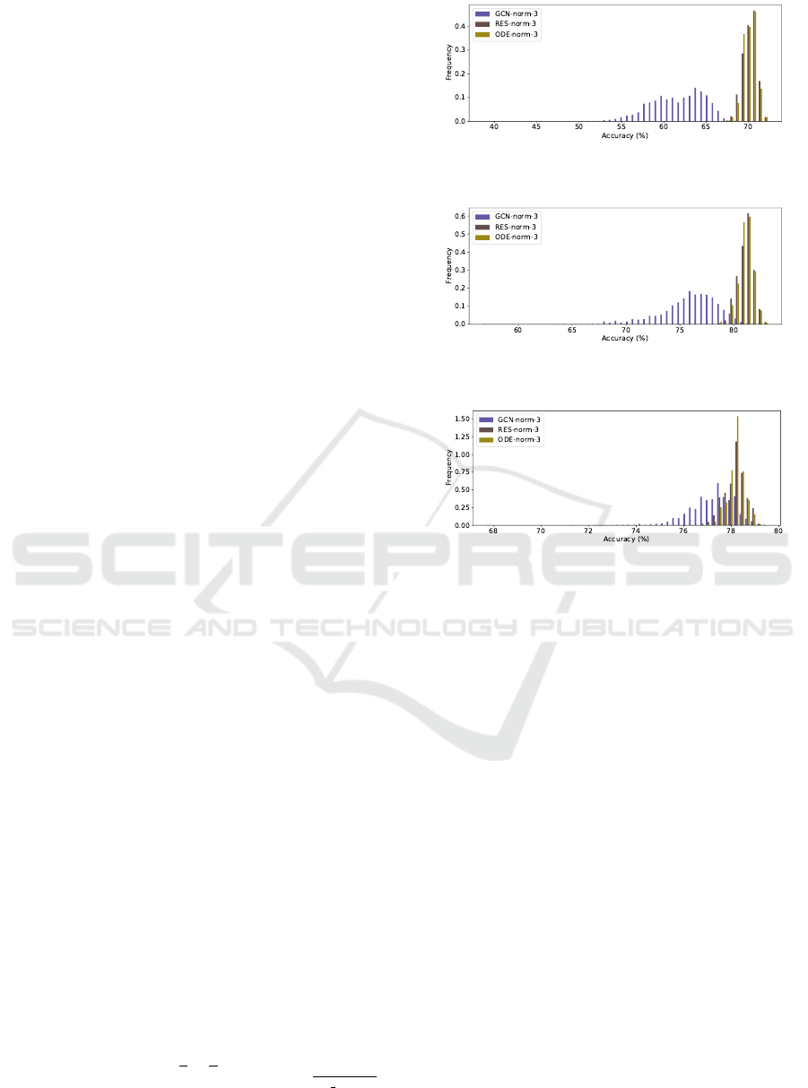
Figure 1: 50-bin histogram of the accuracies, comparing the

models on the Citeseer dataset.

Figure 2: 50-bin histogram of the accuracies, comparing the

models on the Cora dataset.

Figure 3: 50-bin histogram of the accuracies, comparing the

models on the Pubmed dataset.

for accuracy as well as average loss and runtime.

The residual models have a consistently better perfor-

mance, as well as less variance. The residual modules

heavily beneﬁted from group normalisation, however

they were slowed by this addition. The continuous

GCN model achieved the best average accuracy in

Cora and Pubmed, and was close to the best in Cite-

seer. However, it was much slower, partly due to the

group normalisation inside the integrated function.

We tried to train an ODE model with dropout in

the integrated function or without any normalisation,

but it failed to converge in the ﬁrst case and severely

overﬁtted in the second. Even if we consider only the

best over all runs, RES-norm-3 performed better than

any GCN-3 variant, and ODE-norm-3 was less sensi-

tive to weight initialisation, by showing a consistently

lower standard deviation.

To further validate these results, we ran statisti-

cal tests on the accuracies to see whether the differ-

ences between non-residual and residual layers were

statistically signiﬁcant, the p-values for the Mann-

Whitney U-test and Kruskal-Wallis H-test were both

lower than 10

−10

in the Pubmed dataset, and even

lower in the other two, when comparing a resid-

ual (RES, RES-norm and ODE, ODE-norm) module

Discrete and Continuous Deep Residual Learning over Graphs

123

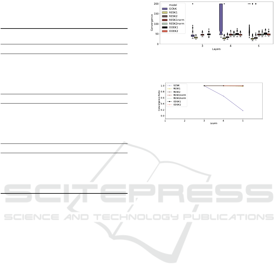
Table 1: Comparison of the performance in the experiments

with 3-layered networks, aggregated as explained in the

text. The best model (except the original) is marked in bold

for each metric.

Model

Acc (%) Loss

Avg Std Min Max Avg

Citeseer

Kipf & Welling 70.30 - - - -

GCN-3 61.70 3.32 37.20 68.80 1.3344

GCN-norm-3 61.66 3.29 38.60 68.70 1.3356

RES-3 65.87 1.46 58.10 70.10 1.1069

RES-norm-3 70.08 0.79 67.40 72.30 1.0132

ODE-norm-3 70.04 0.72 67.50 71.80 1.0163

Cora

Kipf & Welling 81.50 - - - -

GCN-3 76.01 2.59 56.70 81.50 0.8554

GCN-norm-3 75.95 2.68 56.70 81.70 0.8554

RES-3 78.98 1.32 70.60 82.20 0.7114

RES-norm-3 81.06 0.72 78.70 83.20 0.7275

ODE-norm-3 81.08 0.67 78.60 82.70 0.7333

Pubmed

Kipf & Welling 79.00 - - - -

GCN-3 77.19 1.01 68.10 79.30 0.7378

GCN-norm-3 77.19 0.99 67.70 79.30 0.7375

RES-3 77.45 0.77 74.20 79.20 0.7081

RES-norm-3 78.13 0.44 76.10 79.50 0.5602

ODE-norm-3 78.18 0.34 77.20 79.20 0.5602

with a non-residual module (GCN, GCN-norm). The

performance of the discrete and continuous residual

modules was statistically similar, with p-values higher

than 5% for all datasets. Figures 1, 2 and 3 show the

histograms of the accuracies over these runs for each

“norm” model, and can help in visualising that the

residual ones are signiﬁcantly better in average.

4.2 K-layered Models

For the second battery of tests, we present the results

for the Pubmed dataset, since it is the best case for the

baseline non-residual model, as per Figure 3. The “K”

models work in the same way as the “3” models from

Section 4.1, except that they have K layers instead of

3. The residual modules with connections every two

layers had a residual connection on the last layer if

the number of layers is odd. The ODE-solved mod-

ules with residual connections every two layers used

a time component as input to both layers, appended

to every node’s feature vector. All ODE models are

solved using the adjoint method described in (Chen

et al., 2018).

To assess the convergence of the models, we mea-

sure how long it takes for them to meet accuracy and

loss targets, in the validation sets, during training.

Figure 4: Average number of iterations that the models hit

the early stopping criteria in the Pubmed dataset, stopping

at a maximum of 200 epochs.

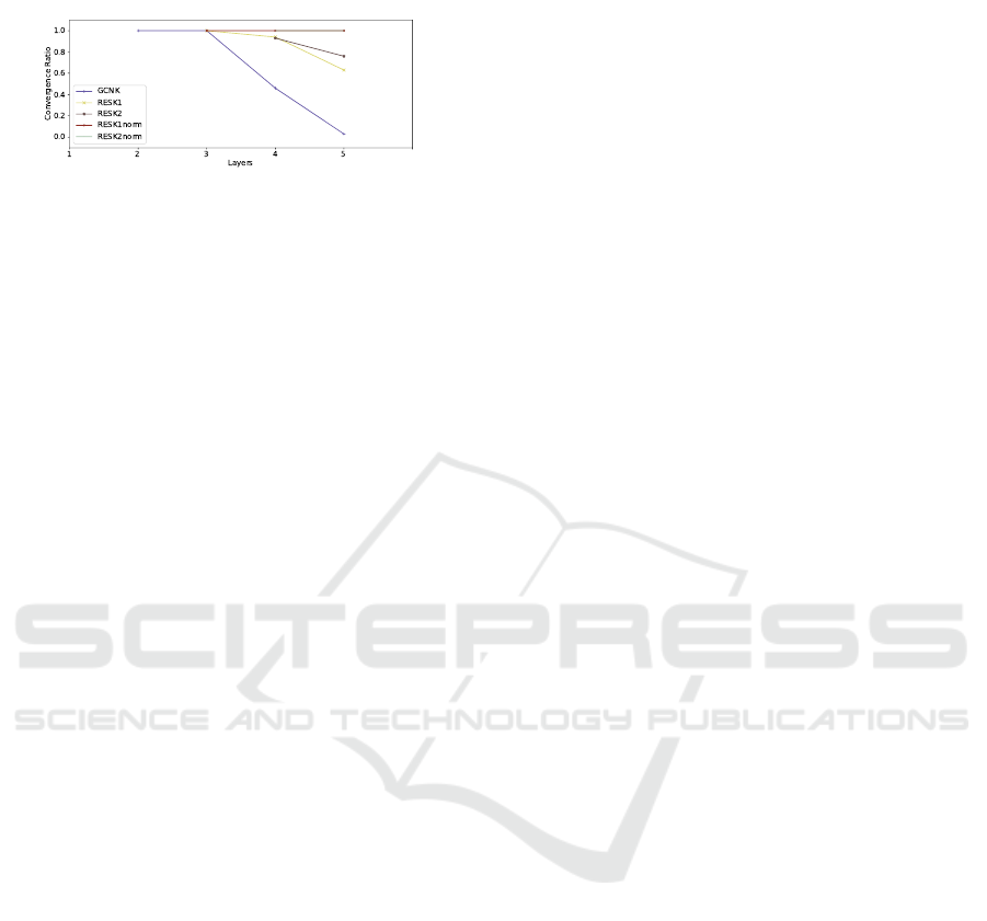
Figure 5: Ratio of models that hit the early stopping criteria

in the Pubmed dataset.

In our early stopping criteria, the target accuracy is

69.47%, which is 90% of the lowest accuracy in Ta-

ble 1, in the Pubmed dataset, whereas the target loss

is 0.78496, which is 110% of the highest test loss ob-

tained in that same test. These targets give the chance

for all models to converge as we know that all of them

could reach those values, when trained with 3 lay-

ers. The reason for using a loss threshold alongside

the accuracy on the validation set is that we wanted

the models to be conﬁdent enough about its predic-

tions and not only accurate. We say that a model did

not converge if it does not stop earlier than the maxi-

mum of 200 training epochs (as proposed in (Kipf and

Welling, 2017)).

Figure 5 shows that the many-layered non-

residual models often failed to converge before the

deﬁned maximum number of epochs. Furthermore,

they had a worse performance when compared to the

residual models. Figure 4 shows that the residual

models hit the early stopping criteria at less than half

the maximum number of iterations, while also some

also show to be more immune or even beneﬁt from

more layers to converge faster. We also ran this ex-

periment for more training iterations and deeper net-

works: the non-residual models were all prone to

overﬁtting while the residual models were more or

less immune to it, achieving good test accuracy even

the earlier stopping criteria was not met.

5 RELATED WORK

Kipf and Welling (Kipf and Welling, 2017) presented

the original GCN formalisation and experimented

ICAART 2021 - 13th International Conference on Agents and Artiﬁcial Intelligence

124

with residual connections, showing that they allow

deeper GCNs. However, experiments with continuous

residual GCN layers, which are the main contribution

of this paper, were not performed. Other papers also

explored the role of residual connections in GNNs,

such as (Bresson and Laurent, 2017; Huang and Car-

ley, 2019), but neither study continuous residual mod-

ules. The application and study of discrete resid-

ual learning over other meta-models has been already

explored in, for example, (Greff et al., 2017; Kim

et al., 2017; Kipf and Welling, 2017; Wang and Tian,

2016; Zilly et al., 2017). Furthermore, the application

of continuous residual learning has been explored in

(Chen et al., 2018; Grathwohl et al., 2018; Haber and

Ruthotto, 2017; Lu et al., 2018; Ruthotto and Haber,

2018), here we found no work applying this tech-

nique to graph-structured data. Independently from

our work a very similar framework, with an almost

equivalent formalisation, was shown in (Poli et al.,

2019) with different results from here, and providing

a complement to this paper.

Many other papers have tried to improve over

(Kipf and Welling, 2017). For example, (Xu et al.,

2019) shows that allowing multiple-layered convolu-

tional kernels improve the expressiveness of the GCN

model, and that the neighbour aggregation method of

the model also impacts on the number of graphs it

can tell apart, proving that a sum aggregation should

be preferred over a mean or max aggregation. Other

work allows attentional pooling of each node’s neigh-

bours (Velickovic et al., 2018), and also show an

improvement in performance. Hamilton, Ying and

Leskovec (Hamilton et al., 2017) experiment with dif-

ferent aggregation/pooling functions for a GCN, and

(Gilmer et al., 2017) uses an edge-annotated pool-

ing in his MPNN. Preliminary experiments with these

models did not yield promising results and thus we

left them for future work, focusing here on the canon-

ical GCN model of (Kipf and Welling, 2017) as our

baseline.

Some models in the GNN literature also employ

methods that can be seen as similar to residual con-

nections. For example, one could interpret the LSTM

and GRU modules, which are often applied in GNNs

(Gilmer et al., 2017; Li et al., 2016; Selsam et al.,

2018), as providing a similar feature to residual con-

nections (Greff et al., 2017), since they may allow in-

formation to pass along time-steps unchanged if the

network learns to do so. Also, (Palm et al., 2018; Xu

et al., 2019) compute the output function in many or

all the layers of their GNN model to perform gradient

descent, instead of performing it only from the end of

the network. This in some sense also allows the gra-

dients to reach speciﬁc parts of the network without

being polluted with further transformations. These

models allow many-layered networks to be effectively

learned and could be seen as having a similar effect to

residual modules, however this is more computation-

ally expensive than allowing residual connections.

6 DISCUSSION

In this paper we provide, to the best of our knowl-

edge, the ﬁrst application of continuous-depth in a

Graph Neural Network. We engineer such a network

by ﬁxing the input graph topology before perform-

ing the integral through an ordinary differential equa-

tion (ODE) solver. This creates a ODE system to be

solved with the input graph’s shape, without using the

matrix as a input parameter to the ODE solver, which

drastically reduces the memory usage. With this, the

learned residual layer applies a continuous operation

through the layer-space, which can behave better than

using discrete transformations on the input.

Although the results we present here do not make

such a strong case for the ODE-solved layers, we be-

lieve this to be mostly due to the problem the origi-

nal GCN paper was applied to and to how the GCN

model itself may act as low-pass ﬁlter (NT and Mae-

hara, 2019). The GCN model performed best with

only two layers, which indicates that the datasets may

not need, and may even be penalised by using, the

information of a larger neighbourhood. We nonethe-

less wanted to present our ﬁrst results with the GCN

model and using the same dataset as the original

paper for two reasons: First, the GCN model pro-

vides and easy-to-bridge intuition between convolu-

tions and GNNs, which helps understand the model

given that the ODE model was also applied to con-

ventional CNNs (Chen et al., 2018), and we wanted

to provide results in the same dataset to provide an

even footing. To achieve an even foooting, however,

we utilised 3-layered models as to allow the resid-

ual modules to learn features intrinsic to their feature

space.

The main advantage we believe that continuous

residual layers can provide on graph-structured data

would be to allow a more predictable behaviour on the

learned functions, as was shown to be the case in other

meta-models in (Chen et al., 2018; Grathwohl et al.,

2018). This would allow complex systems to be mod-

elled as ordinary differential equations, which have a

vast literature of theoretical analysis that could greatly

beneﬁt the Deep Learning community. A prime ex-

ample for such an application would be, for exam-

ple, implementing continuous Interaction Networks

(Battaglia et al., 2016), which would work natively

Discrete and Continuous Deep Residual Learning over Graphs

125

in continuous-time and could be used to better model

physical systems without the errors incurred by sam-

pling.

ACKNOWLEDGEMENTS

We thank NVIDIA Corporation for the Quadro GPU

granted to our research group. We would also like to

thank the Pytorch developers and authors who made

their source code available to foster reproducibil-

ity in research, Henrique Lemos and Rafael Audib-

ert for their helpful discussions and help review-

ing the paper. This study was ﬁnanced in part by

CNPq (Brazilian Research Council) and Coordenac¸

de Aperfeic¸oamento de Pessoal de N

ıvel Superior

(CAPES), Finance Code 001.

REFERENCES

Battaglia, P. W., Hamrick, J. B., Bapst, V., Sanchez-

Gonzalez, A., Zambaldi, V. F., Malinowski, M., Tac-

chetti, A., Raposo, D., Santoro, A., Faulkner, R.,

ulc¸ehre, C¸ ., Song, H. F., Ballard, A. J., Gilmer, J.,

Dahl, G. E., Vaswani, A., Allen, K. R., Nash, C.,

Langston, V., Dyer, C., Heess, N., Wierstra, D., Kohli,

P., Botvinick, M., Vinyals, O., Li, Y., and Pascanu,

R. (2018). Relational inductive biases, deep learning,

and graph networks. CoRR, abs/1806.01261.

Battaglia, P. W., Pascanu, R., Lai, M., Rezende, D. J., and

Kavukcuoglu, K. (2016). Interaction networks for

learning about objects, relations and physics. In NIPS,

pages 4502–4510.

Bresson, X. and Laurent, T. (2017). Residual gated graph

convnets. CoRR, abs/1711.07553.

Chen, T. Q., Rubanova, Y., Bettencourt, J., and Duvenaud,

D. (2018). Neural ordinary differential equations. In

NeurIPS, pages 6572–6583.

Gilmer, J., Schoenholz, S. S., Riley, P. F., Vinyals, O.,

and Dahl, G. E. (2017). Neural message passing for

quantum chemistry. In ICML, volume 70 of Pro-

ceedings of Machine Learning Research, pages 1263–

1272. PMLR.

Glorot, X. and Bengio, Y. (2010). Understanding the dif-

ﬁculty of training deep feedforward neural networks.

In AISTATS, volume 9 of JMLR Proceedings, pages

249–256. JMLR.org.

Gori, M., Monfardini, G., and Scarselli, F. (2005). A new

model for learning in graph domains. In IJCNN, vol-

ume 2, pages 729–734. IEEE.

Grathwohl, W., Chen, R. T. Q., Bettencourt, J., Sutskever, I.,

and Duvenaud, D. (2018). FFJORD: free-form contin-

uous dynamics for scalable reversible generative mod-

els. CoRR, abs/1810.01367.

Greff, K., Srivastava, R. K., and Schmidhuber, J. (2017).

Highway and residual networks learn unrolled itera-

tive estimation. In ICLR (Poster). OpenReview.net.

Haber, E. and Ruthotto, L. (2017). Stable architectures for

deep neural networks. CoRR, abs/1705.03341.

Hamilton, W. L., Ying, Z., and Leskovec, J. (2017). Induc-

tive representation learning on large graphs. In NIPS,

pages 1024–1034.

He, K., Zhang, X., Ren, S., and Sun, J. (2016). Deep resid-

ual learning for image recognition. In CVPR, pages

770–778. IEEE Computer Society.

Hinton, G. E., Srivastava, N., Krizhevsky, A., Sutskever,

I., and Salakhutdinov, R. (2012). Improving neural

networks by preventing co-adaptation of feature de-

tectors. CoRR, abs/1207.0580.

Huang, B. and Carley, K. M. (2019). Residual or

gate? towards deeper graph neural networks for

inductive graph representation learning. CoRR,

abs/1904.08035.

Kim, J., El-Khamy, M., and Lee, J. (2017). Residual

LSTM: design of a deep recurrent architecture for dis-

tant speech recognition. In INTERSPEECH, pages

1591–1595. ISCA.

Kipf, T. N. and Welling, M. (2017). Semi-supervised clas-

siﬁcation with graph convolutional networks. In ICLR

(Poster). OpenReview.net.

Li, Q., Han, Z., and Wu, X. (2018). Deeper insights into

graph convolutional networks for semi-supervised

learning. In AAAI, pages 3538–3545. AAAI Press.

Li, Y., Tarlow, D., Brockschmidt, M., and Zemel, R. S.

(2016). Gated graph sequence neural networks. In

ICLR (Poster).

Lu, Y., Zhong, A., Li, Q., and Dong, B. (2018). Beyond

ﬁnite layer neural networks: Bridging deep architec-

tures and numerical differential equations. In ICML,

volume 80 of Proceedings of Machine Learning Re-

search, pages 3282–3291. PMLR.

NT, H. and Maehara, T. (2019). Revisiting graph neural

networks: All we have is low-pass ﬁlters. CoRR,

abs/1905.09550.

Palm, R. B., Paquet, U., and Winther, O. (2018). Recurrent

relational networks. In NeurIPS, pages 3372–3382.

Poli, M., Massaroli, S., Park, J., Yamashita, A., Asama, H.,

and Park, J. (2019). Graph neural ordinary differential

equations. CoRR, abs/1911.07532.

Ruthotto, L. and Haber, E. (2018). Deep neural networks

motivated by partial differential equations. CoRR,

abs/1804.04272.

Scarselli, F., Gori, M., Tsoi, A. C., Hagenbuchner, M.,

and Monfardini, G. (2009). The graph neural net-

work model. IEEE Transactions on Neural Networks,

20(1):61–80.

Selsam, D., Lamm, M., B

unz, B., Liang, P., de Moura, L.,

and Dill, D. L. (2018). Learning a SAT solver from

single-bit supervision. CoRR, abs/1802.03685.

Veit, A., Wilber, M. J., and Belongie, S. J. (2016). Residual

networks behave like ensembles of relatively shallow

networks. In NIPS, pages 550–558.

Velickovic, P., Cucurull, G., Casanova, A., Romero, A., Li

P., and Bengio, Y. (2018). Graph attention networks.

In ICLR (Poster). OpenReview.net.

Wang, Y. and Tian, F. (2016). Recurrent residual learning

for sequence classiﬁcation. In EMNLP, pages 938–

943. The Association for Computational Linguistics.

Wu, Y. and He, K. (2018). Group normalization. In ECCV

(13), volume 11217 of Lecture Notes in Computer Sci-

ence, pages 3–19. Springer.

ICAART 2021 - 13th International Conference on Agents and Artiﬁcial Intelligence

126

Wu, Z., Pan, S., Chen, F., Long, G., Zhang, C., and Yu,

P. S. (2019). A comprehensive survey on graph neural

networks. CoRR, abs/1901.00596.

Xu, K., Hu, W., Leskovec, J., and Jegelka, S. (2019). How

powerful are graph neural networks? In ICLR. Open-

Review.net.

Yang, Z., Cohen, W. W., and Salakhutdinov, R. (2016). Re-

visiting semi-supervised learning with graph embed-

dings. In ICML, volume 48 of JMLR Workshop and

Conference Proceedings, pages 40–48. JMLR.org.

Zilly, J. G., Srivastava, R. K., Koutn

ık, J., and Schmidhuber,

J. (2017). Recurrent highway networks. In ICML,

volume 70 of Proceedings of Machine Learning Re-

search, pages 4189–4198. PMLR.

APPENDIX

Detailed Model and Experiments

Experiments

The experiments we run are the same as those pre-

sented in (Kipf and Welling, 2017). We use the same

train/test/evaluation split as they use, which was in-

herited from (Yang et al., 2016).

Models

For our experiments we used a slightly different ver-

sion of the proposed GCN model, which follows

Equation 10 instead of the original one. Similarly, the

discrete residual module follows Equation 11, and the

continuous one approximates Equation 12.

l+1

= σ(

−1

) (10)

l+1

= σ(

−1

) (11)

δH(l)

δl

= σ(

−1

AH(l)W (l)) (12)

All the tested models use either dropout (Hinton et al.,

2012), group normalisation (Wu and He, 2018) (or

both), and L2 normalisation of the parameters are de-

scribed as follows:

GCN-3. A model with the GCN layer as made avail-

able by the author, with dropout applied between

each pair of layers.

RES-3. A model with a residual GCN kernel as de-

ﬁned in Equation 11 instead of a normal GCN on

the second layer, with dropout applied between

each pair of layers.

GCN-norm-3. A model with the GCN layer as made

available by the author, with dropout applied be-

tween the ﬁrst and second layer and group nor-

malisation applied between the second and the

third.

RES-norm-3. A model with a residual GCN ker-

nel as deﬁned in Equation 11 instead of a nor-

mal GCN on the second layer, with dropout ap-

plied between the ﬁrst and second layer and group

normalisation applied between the second and the

third.

RES-fullnorm-3. A model with a residual GCN ker-

nel as deﬁned in Equation 11 instead of a normal

GCN on the second layer, with group normalisa-

tion applied between each pair of layers.

ODE-norm-3. A model with a continuous residual

module as deﬁned in Equation 12 instead of a nor-

mal GCN on the second layer, dropout before the

ODE-solved layer and group normalisation as part

of the ODE-solved layer, applied to its input. The

ODE-solved layers use the technique described in

Subsection 3.4 to allow the learned continuous

transformation to be dependant on the time pa-

rameter evaluations.

ODE-fullnorm-3. A model with a continuous resid-

ual module as deﬁned in Equation 12 instead of a

normal GCN on the second layer, group normal-

isation both before the ODE-solved layer and as

part of the ODE-solved layer, applied to its in-

put. The ODE-solved layers use the technique

described in Subsection 3.4 to allow the learned

continuous transformation to be dependant on the

time parameter evaluations.

All models use 16 features in all their hidden dimen-

sions, which was kept from the original code as the

default, since (Velickovic et al., 2018) showed that

increasing the number of features did not seem to im-

prove performance on the GCN. All learned kernels

weights are initialised with the uniform distribution

U(−

√

k), where k =

out features

and their biases

are also initialised from the same distribution.

The “K” models work in the same way as the “3”

models, only that they have K layers instead of 3,

with the normalisation between the ﬁrst and second

layer being the same, and on the other layers being

the same as the normalisation between the second and

third layer in the “3” model. All models had ReLU ac-

tivations after every layer but the last, applied before

the normalisation. On the last layer all models had a

log softmax applied to each node’s output. The resid-

ual modules with connections every two layers had a

residual connection on the last layer if the number of

layers is odd. The ODE-solved modules with residual

connections every two layers used a time component

as input both layers, appended to every node’s feature

vector. All ODE models are solved using the adjoint

method described in (Chen et al., 2018).

To perform neighbourhood aggregation we ran

Discrete and Continuous Deep Residual Learning over Graphs

127

Pytorch’s sparse matrix multiplication (torch.spmm)

between the degree-normalised adjancency matrix

and the nodes features, essentially doing a weighted

sum through all the neighbours, with all weights set

to 1/d

where d

is the degree for node n.

Additional Results

Full Results for 3-layered Models

In this section we present the full results of the ex-

periments done in the corresponding section of the

paper. For implementation notes on the models look

at Appendix 6. Table 2 shows the average, standard

deviation and the best and worst values over all the

runs for accuracy as well as average loss and run-

time. There one can see that the residual models have

a consistently better performance, as well as less vari-

ance in the range of possible accuracies. The mod-

els trained in this work are, as stated in the provided

source, “subtly different” from the ones presented in

the original paper, and the author stated that the code

we adapted does not fully reproduce the results in the

paper.

We made statistical tests to with the null-

hipothesis of a pair of models being similar, the p-

values for the Mann-Whitney U-test and Kruskal-

Wallis H-test were both lower than 10

−10

in the

Pubmed dataset, and even lower in the other two,

when comparing a residual (RES, RES-norm and

ODE, ODE-norm) module with a non-residual mod-

ule (GCN, GCN-norm). When comparing the two

residual modules the null hypothesis was not rejected,

with p-values higher than 5% for all datasets. Fig-

ures 7, 6 (Also presented in the paper) and 8 show

the histograms of the accuracies over these runs for

each “norm” model, and can help in visualising that

the residual ones are signiﬁcantly better in average.

K-layered Models and Discussion

For the second battery of tests, we present the re-

sults for the Cora dataset in Figures 9, 10, 11, for

the Pubmed dataset in Figures 12, 13, 14, and the

additional ﬁgure for the Citeseer dataset in Figure

15. One of the points which caused degradation with

the stacking of more layers is that we also put a loss

threshold in the early stopping, causing some of the

models to overﬁt the data. The reason for using a

loss threshold along the accuracy on the validation set

is that we wanted our model to be conﬁdent enough

about its predictions and not only accurate. We also

ran this experiment for a larger number of layers and

the results seemed stable throughout, we chose to

present here only from layers 3 through 5 since in this

Table 2: Comparison of the performance in the reproduction

of the experiments done in (Kipf and Welling, 2017). The

experiments were run 2500 times for the non-continuous

models (those that don’t start with “ODE”), and 250 times

for the continuous ones. The results shown here are the av-

erage, standard deviation, minimum and maximum of these

runs to minimise the effect of the variables’ random initiali-

sation. Runtime isn’t comparable with different setups, and

is presented for the original paper only for completeness.

GCN (Paper) represents that the results were taken from

(Kipf and Welling, 2017).

Model

Acc (%) Loss Time (s)

Avg Std Min Max Avg Avg

Citeseer

GCN (Paper) 70.30 - - - - 7

GCN-3 61.70 3.32 37.20 68.80 1.3344 1.4325

GCN-norm-3 61.66 3.29 38.60 68.70 1.3356 1.4399

RES-3 65.87 1.46 58.10 70.10 1.1069 1.4480

RES-norm-3 70.08 0.79 67.40 72.30 1.0132 2.2851

RES-fullnorm 16.17 4.99 7.70 23.10 1.7918 3.1579

ODE-norm-3 70.04 0.72 67.50 71.80 1.0163 69.7444

ODE-fullnorm-3 18.28 2.59 16.00 23.10 1.7918 61.0533

Cora

GCN (Paper) 81.50 - - - - 4

GCN-3 76.01 2.59 56.70 81.50 0.8554 1.3841

GCN-norm-3 75.95 2.68 56.70 81.70 0.8554 1.3944

RES-3 78.98 1.32 70.60 82.20 0.7114 1.3888

RES-norm-3 81.06 0.72 78.70 83.20 0.7275 2.0943

RES-fullnorm 15.07 8.87 6.40 31.90 1.9459 2.7927

ODE-norm-3 81.08 0.67 78.60 82.70 0.7333 62.2312

ODE-fullnorm-3 14.09 6.49 6.40 31.90 1.9458 54.8411

Pubmed

GCN (Paper) 79.00 - - - - 38

GCN-3 77.19 1.01 68.10 79.30 0.7378 5.6163

GCN-norm-3 77.19 0.99 67.70 79.30 0.7375 5.6146

RES-3 77.45 0.77 74.20 79.20 0.7081 5.6194

RES-norm-3 78.13 0.44 76.10 79.50 0.5602 10.5187

RES-fullnorm 32.82 11.11 18.00 41.30 1.0986 15.4539

ODE-norm-3 78.18 0.34 77.20 79.20 0.5602 346.6378

ODE-fullnorm-3 36.40 9.20 18.00 41.30 1.0986 289.2936

range the performance degradation of non-residual

GCNs is already visible.

Note that all the experiments we’ve done here,

with 3-layered networks, perform slightly worse than

a 2-layered network in most datasets. The original

paper already shows that this seems to be the opti-

mal number of layers for this dataset, and in the orig-

inal paper they used a different kernel initialization

method. The main point of our experiments was to

show the immunity of the residual networks to the

number of layers and initial parameter intialisation.

We trained a 2-layered discrete residual network, tak-

ing only a slice of the output of the layer as the ﬁ-

nal features

, this model performed similarly to the

non-residual module, and achieved performance near

to the one presented in the original paper. Also, the

two-layered networks couldn’t take advantage of the

group normalisation technique, and were slightly less

scientiﬁcally interesting to analyse because of this.

This was done so that the layer has the same number of

in and out features.

ICAART 2021 - 13th International Conference on Agents and Artiﬁcial Intelligence

128

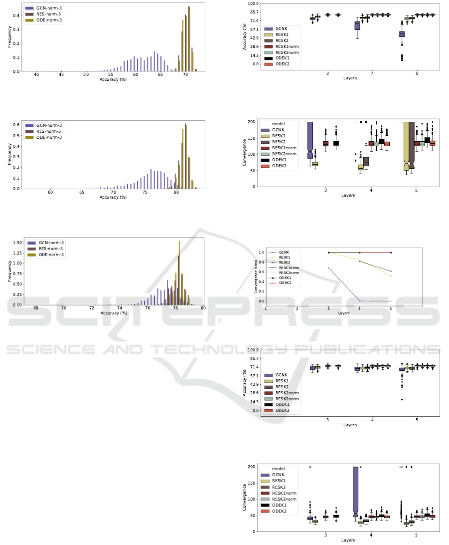
Figure 6: 50-bin histogram of the accuracies, comparing the

models on the Citeseer dataset.

Figure 7: 50-bin histogram of the accuracies, comparing the

models on the Cora dataset.

Figure 8: 50-bin histogram of the accuracies, comparing the

models on the Pubmed dataset.

Other Experiments on the Citation Networks

We also preliminarly trained GCNs on the Cora

dataset, using sum neighbour aggregation instead of

mean aggregation. These performed slightly worse

than mean aggregation. Furthermore, the residual lay-

ers suffered in their performance without group nor-

malisation for many-layered networks when sum ag-

gregation was used. With this in mind, we disregarded

the use of sum aggregation for GCNs for our exper-

iments. We used MLPs instead of linear layers for

the convolutional kernels, but the performance did not

seem to increase as well.

Another difference between what we present here

and the results originally published (one of the parts

where the code we used was “subtly different” from

the one which produced the published results) is that

the original paper used a different kernel initialisa-

tion, using the Xavier/Glorot initialisation described

in (Glorot and Bengio, 2010). We tested the mod-

els with the Glorot initialisation, the results of which

can be seen in Table 3, where we ran the models for

only 100 runs. Still, the models we trained seemed to

slightly underperform the results shown in the origi-

Figure 9: Average ﬁnal test accuracy of the models in the

Cora dataset.

Figure 10: Average number of iterations that the models hit

the early stopping criteria in the Cora dataset, stopping at a

maximum of 200 epochs.

Figure 11: Ratio of models that hit the early stopping crite-

ria in the Cora dataset.

Figure 12: Average ﬁnal test accuracy of the models which

hit the early stopping criteria in the Pubmed dataset.

Figure 13: Average number of iterations that the models hit

the early stopping criteria in the Pubmed dataset, stopping

at a maximum of 200 epochs.

nal paper. We also experimented using dense matrices

for the adjacencies which did not provide any perfor-

mance boost.

Discrete and Continuous Deep Residual Learning over Graphs

129

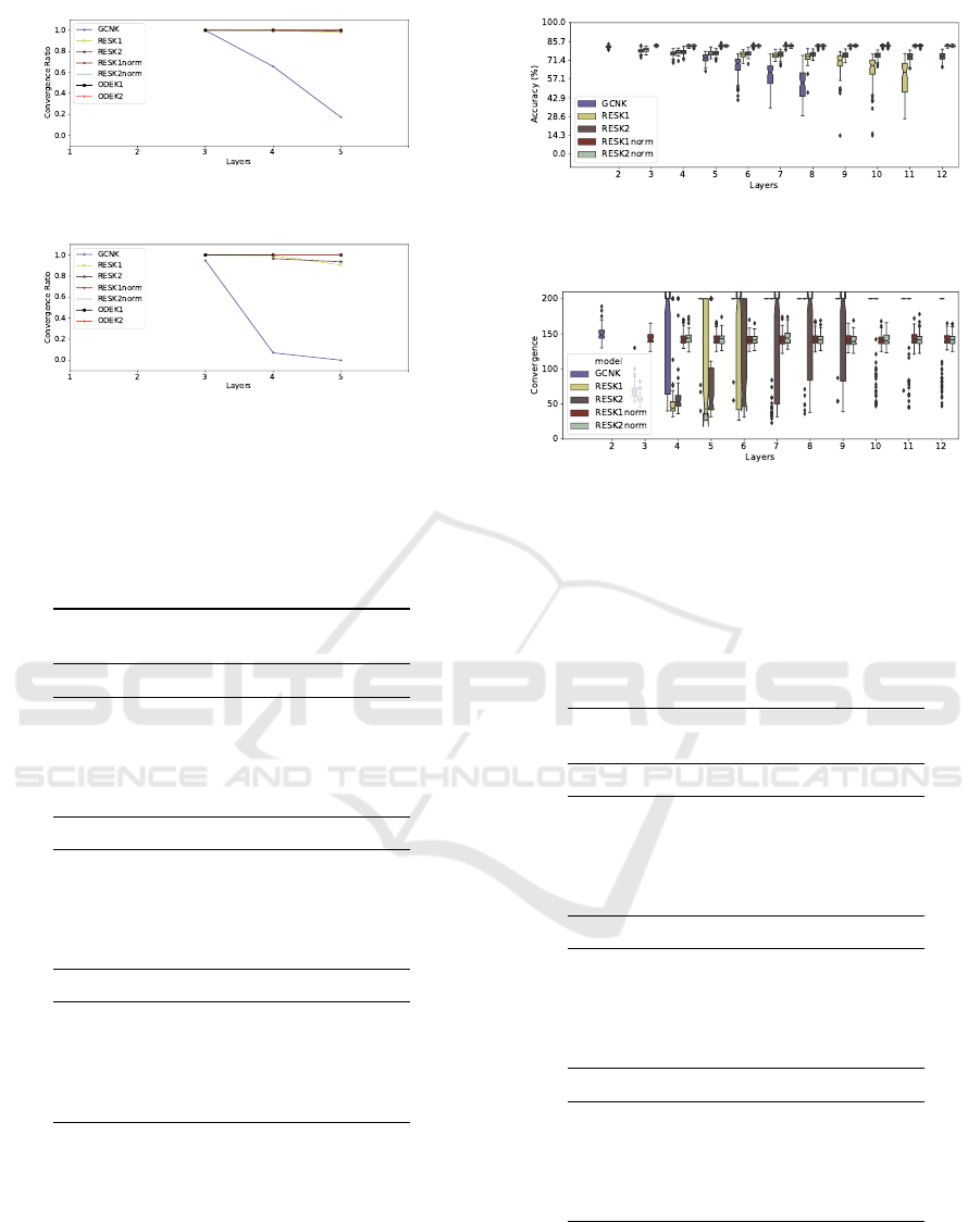
Figure 14: Ratio of models that hit the early stopping crite-

ria in the Pubmed dataset.

Figure 15: Ratio of models that hit the early stopping crite-

ria in the Citeseer dataset.

Table 3: Comparison of the performance in the reproduction

of the experiments done in (Kipf and Welling, 2017). The

experiments were run 100 times for all models. The results

shown here are the average, standard deviation, minimum

and maximum of these runs. GCN (Paper) represents that

the results were taken from (Kipf and Welling, 2017).

Model

Acc (%) Loss

Avg Std Min Max Avg

Citeseer

GCN (Paper) 70.30 - - - -

GCN-3 65.18 1.78 61.40 69.80 1.1817

GCN-norm-3 65.33 1.93 56.40 70.10 1.1728

RES-3 66.46 1.41 62.70 69.70 1.1190

RES-norm-3 70.15 0.67 68.10 71.60 0.9908

Cora

GCN (Paper) 81.50 - - - -

GCN-3 78.87 1.40 75.30 82.00 0.7391

GCN-norm-3 78.44 1.36 74.10 80.90 0.7557

RES-3 79.19 1.24 75.40 81.80 0.7159

RES-norm-3 80.98 0.73 79.00 83.10 0.7022

Pubmed

GCN (Paper) 79.00 - - - -

GCN-3 77.15 0.77 75.00 78.60 0.7474

GCN-norm-3 77.25 0.88 74.30 79.00 0.7467

RES-3 77.38 0.83 75.20 78.80 0.7314

RES-norm-3 78.05 0.42 76.80 78.90 0.5577

Having done this, we tried following the paper as

closely as possible, using the Xavier/Glorot initiali-

sation (Glorot and Bengio, 2010), dropout in the in-

put. The results for this can in Table 4, where we ran

the models for only 100 runs. The 2-layered GCN

model achieved the same performance as in the orig-

inal paper and the null hypothesis was rejected when

comparing the GCN model to the ODE model, with

the ODE model being slightly inferior than the GCN

Figure 16: Average ﬁnal test accuracy of the models which

hit the early stopping criteria in the Cora dataset by follow-

ing the paper more closely.

Figure 17: Average number of iterations that the models hit

the early stopping criteria in the Cora dataset by follow-

ing the paper more closely, stopping at a maximum of 200

epochs.

Table 4: Comparison of the performance in the reproduction

of the experiments done in (Kipf and Welling, 2017). The

experiments were run 100 times for all models. The results

shown here are the average, standard deviation, minimum

and maximum of these runs.

Model

Acc (%) Loss

Avg Std Min Max Avg

Citeseer

GCN-3 65.71 2.04 55.60 69.10 1.1202

GCN-norm-3 65.49 1.98 56.50 69.30 1.1306

RES-3 66.78 1.39 63.10 69.80 1.0776

RES-norm-3 70.75 0.85 68.50 73.00 1.0433

ODE-norm-3 69.51 1.09 67.30 72.10 1.0616

Cora

GCN-3 79.41 1.52 75.80 82.80 0.6776

GCN-norm-3 79.59 1.46 75.70 82.20 0.6748

RES-3 80.33 1.21 77.90 82.80 0.6469

RES-norm-3 81.87 0.70 80.10 83.50 0.7710

ODE-norm-3 81.52 0.75 79.20 83.10 0.7841

Pubmed

GCN-3 77.49 0.78 75.20 79.00 0.7063

GCN-norm-3 77.41 0.88 75.30 79.00 0.7121

RES-3 77.59 0.87 75.30 79.20 0.6924

RES-norm-3 79.11 0.60 77.20 80.10 0.5679

ODE-norm-3 78.50 0.47 77.20 79.80 0.5904

model. One can also look at Figures 16, 17, and 18

for results similar to the ones discussed in the other

sections for the Cora dataset. These changes also in-

crease the number of layers the non-residual model

can be built with before its performance degrades too

ICAART 2021 - 13th International Conference on Agents and Artiﬁcial Intelligence

130

much.

Figure 18: Ratio of models that hit the early stopping crite-

ria in the Cora dataset by following the paper more closely.

Discrete and Continuous Deep Residual Learning over Graphs

131