Analysis of Feature Representations

for Anomalous Sound Detection

Robert M

uller

, Steffen Illium

, Fabian Ritz

and Kyrill Schmid

Mobile and Distributed Systems Group, LMU Munich, Germany

Keywords:

Anomaly Detection, Transfer Learning, Machine Health Monitoring.

Abstract:

In this work, we thoroughly evaluate the efﬁcacy of pretrained neural networks as feature extractors for anoma-

lous sound detection. In doing so, we leverage the knowledge that is contained in these neural networks to

extract semantically rich features (representations) that serve as input to a Gaussian Mixture Model which is

used as a density estimator to model normality. We compare feature extractors that were trained on data from

various domains, namely: images, environmental sounds and music. Our approach is evaluated on recordings

from factory machinery such as valves, pumps, sliders and fans. All of the evaluated representations outper-

form the autoencoder baseline with music based representations yielding the best performance in most cases.

These results challenge the common assumption that closely matching the domain of the feature extractor and

the downstream task results in better downstream task performance.

1 INTRODUCTION

In the emerging ﬁeld of anomalous sound detection

(ASD), one aims to develop computational meth-

ods to reliably detect anomalies in acoustic sounds.

These methods can be considered as the counterpart

to anomaly detection on visual data and are used in

situations where visual monitoring is infeasible. One

of the most important use-cases is the early detection

of malfunctions during the operation of factory ma-

chinery. A robust ASD system reduces repair costs,

improves safety and prevents consequential damages

by enabling early maintenance. Moreover, it reduces

the ﬁnancial burden, an aspect that becomes increas-

ingly important considering the rising costs of modern

machinery and equipment.

While our work focuses on the scenario above,

other ASD systems have been developed for closely

related applications such as monitoring production

processes for irregularities (Hasan et al., 2018), the

detection of leaks in water supply networks (M

uller

et al., 2020a) and sound-based security systems for

public spaces (Hayashi et al., 2018).

Since it is expensive and tedious to collect an

https://orcid.org/0000-0003-3108-713X

https://orcid.org/0000-0003-0021-436X

https://orcid.org/0000-0001-7707-1358

https://orcid.org/0000-0001-6748-4896

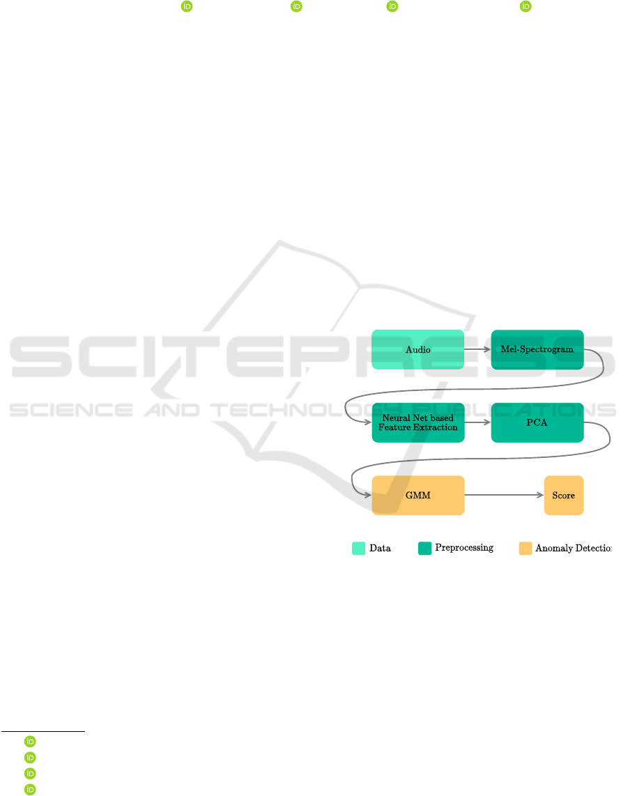
Figure 1: High-Level overview of the proposed workﬂow.

exhaustive number of anomalous samples that cover

all possible anomalies in such settings, training ASD

models is usually carried out on normal operation data

only to learn a notion of normality. Moreover, even if

it was possible to collect large amounts of anomalous

data, some anomalies might not even be known be-

forehand and are thus not available during training.

Most of the recent ASD approaches rely on deep

autoencoders (AEs). AEs ﬁrst compress their in-

put into a low dimensional latent code using an en-

coder neural network (NN). This code is subsequently

used to reconstruct the input with a decoder network.

Hence, AEs do not use external labels. It is assumed

Müller, R., Illium, S., Ritz, F. and Schmid, K.

Analysis of Feature Representations for Anomalous Sound Detection.

DOI: 10.5220/0010226800970106

In Proceedings of the 13th International Conference on Agents and Artiﬁcial Intelligence (ICAART 2021) - Volume 2, pages 97-106

ISBN: 978-989-758-484-8

that patterns seen during training yield a lower re-

construction error than those not seen during train-

ing. Consequently the reconstruction error is used as a

measure of abnormality. However, AEs proposed for

ASD have to be trained from scratch and do not use

prior information or leverage additional training data

from other domains. Due to the widespread avail-

ability of acoustic datasets and NNs that were trained

on related tasks such as environmental sound clas-

siﬁcation, the question arises whether their knowl-

edge, obtained from tasks for which a large amount

of data is available, can be transferred and exploited

to increase ASD performance. This approach is com-

monly referred to as Transfer Learning.

Transfer learning is mainly used in computer vi-

sion and natural language processing (NLP) but has

also started to gain traction in acoustic signal process-

ing.

In computer vision, it is common to ﬁne-tune a

neural network that was pre-trained on ImageNet for

the task of image classiﬁcation e.g. by only chang-

ing some of the last layers and ﬁne-tuning the net-

work on a downstream task. Another approach is to

extract some of the activations (e.g. from the penul-

timate dense layer) of the pretrained network and use

them as feature vectors that serve as input to more

traditional (e.g. shallow, linear) models. Note that in

this case the pretrained network is solely used as fea-

ture extractor and its weights are not updated through

gradient descent. In both cases, transfer learning con-

siderably reduces the amount of training data needed

for the downstream task (Donahue et al., 2014).

In NLP, the advent of pretrained language mod-

els has lead to substantial improvements on a wide

range of tasks (Ruder, 2018). Almost all modern

approaches rely on some sort of pretrained (word)

representations or networks. Recent approaches are

trained on (masked) language modeling and use trans-

former (Devlin et al., 2019) or recurrent neural net-

work architectures (Peters et al., 2018). In the ﬁrst

stage the models are trained to solve the very general

task of understanding natural language. Afterwards

the NNs are ﬁne-tuned or simply used as feature ex-

tractors to solve tasks such as sentiment analysis and

machine translation.

Finally, there exist several pretrained networks

from the ﬁeld of acoustic signal processing. For ex-

ample, (Chi et al., 2020) use a transformer based

architecture to predict masked Mel-spectrogram

frames to obtain contextualized speech representa-

tions. (Beckmann et al., 2019) adopt the classic VGG-

16 architecture on a spoken word classiﬁcation task

to obtain transferable representations. (Cramer et al.,

2019) propose a self-supervised audio-visual corre-

spondence task and use the resulting features in con-

junction with a simple two layer neural network to

achieve state-of-the-art performance for environmen-

tal sound classiﬁcation.

Despite of their easy availability, these networks

are rarely used in other work i.e. most models are

trained from scratch and the possible beneﬁts that the

inclusion of pretrained NNs could provide are ne-

glected.

In this work, we aim to evaluate the effectiveness

of transferring knowledge from related domains us-

ing different pretrained NNs for the task of anomalous

sound detection. Since no labels are available in ASD,

we follow the feature extraction paradigm in conjunc-

tion with a Gaussian Mixture Model (GMM). We hy-

pothesize that using the right representation in con-

junction with a simple anomaly detection algorithm

rivals the performance of the currently widely used

autoencoder. We evaluate our approach with repre-

sentations from three different domains chosen due

to their structural similarity with machine sounds: (i)

Image based representations (ii) Environmental sound

based representations (iii) Music based representa-

tions. From a practical point of view, this approach

allows for fast experiments as only shallow models

have to be trained and alleviates the burden of design-

ing a suitable neural network architecture and training

task.

We show that all representations outperform the

autoencoder baseline (Kawaguchi et al., 2019) in

terms of ASD performance. The best results are ob-

tained with music based representations. To the best

of our knowledge, this is the ﬁrst study that thor-

oughly evaluates the efﬁcacy of different feature rep-

resentations for anomalous sound detection.

The rest of the paper is structured as follows: In

Section 2 we brieﬂy review related work followed by

a discussion of our ASD approach in Section 3. Then

we go on to describe the experimental setup and the

dataset we used to evaluate our approach in Section 4.

The results are discussed in Section 5. We close by

summarizing our ﬁndings and outlining future work

in Section 6.

2 RELATED WORK

As stated before, the majority of approaches to

anomalous sound detection uses deep autoencoders.

(Duman et al., 2019) use a convolutional AE to recon-

struct Mel-spectrograms in order to detect anomalies

in industrial plants. (Koizumi et al., 2017) concate-

nate several spectrogram frames as input to a simple,

densly connected autoencoder. Here ASD is consid-

ICAART 2021 - 13th International Conference on Agents and Artiﬁcial Intelligence

ered as a statistical hypothesis test where they pro-

pose a loss function based on the Neyman-Pearson

lemma. However this approach relies on the simula-

tion of anomalous sounds using expensive rejection

sampling. (Suefusa et al., 2020) use a similar AE

architecture to predict the center frame from the re-

maining frames. This is based upon the observation

that the edge frames are usually harder to reconstruct,

especially when dealing with non-stationary sounds.

(Marchi et al., 2015; Bayram et al., 2020) account

for the sequential nature of sound and use sequence-

to-sequence network architectures to reconstruct au-

ditory spectral features.

A slightly different approach is taken

by (Kawaguchi et al., 2019). Here an ensemble

of simple autoencoders is used for ASD. Various

acoustic front-end algorithms are applied for rever-

beration and denoising to preprocess the data. This

improves performance as the AEs are freed from the

burden of reconstructing noise.

SNIPER (Koizumi et al., 2019) is a novel way to

incorporate anomalies that were overlooked during

operation without retraining the whole system. For

each overlooked anomaly, a new detector is cascaded

that is constrained to have a true positive rate (TPR)

= 1 for that speciﬁc anomaly. To compute the TPR,

a generative model is used to simulate samples of the

observed anomaly.

Apart from spectrogram based approaches a few

ASD approaches that directly operate on the wave-

form have been developed (Hayashi et al., 2018;

Rushe and Namee, 2019). These methods use causal

dilated convolutions (Oord et al., 2016) to predict the

next sample, i.e. they are autoregressive models that

use the prediction error to measure abnormality.

3 ASD APPROACH

In this section, we brieﬂy introduce the common

acoustic signal processing workﬂow. Then we de-

scribe our ASD appraoch that relies upon pretrained

NNs for feature extraction and Gaussian Mixture

Models for density estimation in more detail.

Most machine learning models do not directly operate

on the raw waveform i.e. a sequence of air pressure

measurements. Instead, it is ﬁrst transformed from

the time domain to the frequency domain exploiting

the fact that arbitrarily complex waves can be repre-

sented as a combinations of simple sinusoids. In prac-

tice, this is done using the short-time-fourier trans-

form (STFT). The STFT simply applies the discrete-

fourier-transform on small overlapping chunks of the

raw signal to account for signals whose frequency

characteristics change over time.

The output of the STFT is a matrix S ∈ R

F×T

with

F frequency bins and T time frames and is called the

spectrogram. Each cell represent the amplitude (the

normalized squared magnitude) of the corresponding

frequency bin at some point in time.

To account for the fact that the human perception of

pitch is logarithmic in nature, i.e. humans are more

discriminative at lower frequencies and less discrim-

inative at higher frequencies, one additionally trans-

forms the frequency bins into the Mel-scale using the

Mel-ﬁlterbank that is composed of overlapping trian-

gular ﬁlters. The Mel-scale is an empirically deﬁned

perceptual scale that mirrors human perception. Fil-

ters are small for low frequencies and are of increas-

ing width for higher frequencies. They aggregate the

energy of consecutive frequency bins to describe how

much energy exists in various frequency regions. This

can be seen as a re-binning procedure that alters the

number of bins from F to M , M < F where M is

the number of Mel-ﬁlters used. Finally the log of the

energies is taken to convert from amplitude to decibel

(dB). The resulting Mel-spectrogram is a compact vi-

sual representation of audio that can be used as input

to a machine-learning pipeline. Moreover, the Mel-

spectrogram can be treated as an image of the under-

lying signal and one can therefore resort to computer

vision approaches such as convolutional neural net-

works (CNNs).

We assume that the ASD system monitors the entity

for an application speciﬁc, predeﬁned period of time

(decision horizon) until the degree of abnormality (or

normality) needs to be estimated and that we are given

a dataset of normal operation recordings only. There-

fore, we assume that the dataset D is a set of n (equal-

length) Mel-spectrograms

D = M

,... ,M

∈ R

M ×T

(1)

where T is proportional to the decision horizon.

It is common to subdivide the computation of the ﬁ-

nal anomaly score into a sequence of smaller predic-

tions that operate on a smaller timescale. For exam-

ple, the decision horizon might be 10 seconds but the

ASD system outputs an anomaly score every 0.5 sec-

onds. This is a simple strategy to avoid overlook-

ing subtle short-term anomalies and causes a trade-

of between local and global structure. A score for

the whole decision horizon is obtained by aggrega-

tion. In our case, we transform each Mel-spectrogram

, i = 1 . .. n into a sequence of feature representa-

tions V

∈ R

D×

by using a sliding window across

the columns (time dimension). For each window of

t frames, a feature extractor

Φ : R

M ×t

→ R

(2)

Analysis of Feature Representations for Anomalous Sound Detection

extracts a D dimensional feature vector that is more

semantically compact than raw Mel-spectrogram fea-

tures. Furthermore, the feature extractor leverages

prior knowledge obtained through its pretext task.

Then the window is moved h frames to the right. Con-

sequently, the transformed dataset D

has the form

= V

,. .. ,V

∈ R

D×

(3)

The number of feature vectors

T is given by

T −n

Note that if

T −n

6∈ N an appropriate padding strategy

has to be applied.

Since no labels are available we propose to ﬁt a Gaus-

sian mixture model (GMM) with K components to in-

dividual feature vectors in order to being able to com-

pute their density. The density can in turn be used to

describe the degree of normality of a single feature

vector.

The GMM was chosen as anomaly detector as it was

shown (M

uller et al., 2020b) to outperform other

models on the task of anomalous sound detection

when using image based features. Moreover, GMMs

are fast and easy to train due to the ready availability

of reliable implementations, have a sound probabilis-

tic interpretation and have the capability to model ar-

bitrary densities.

The density of a single feature vector x ∈ R

is given

by:

p(x) =

∑

k=1

∗ N(x|µ

,Σ

) (4)

, Σ

and λ

are the mean, covariance matrix

and weight of the kth mixture component where

∑

k=1

= 1. We compute the anomaly score for some

as follows:

p(V

) = p(V

i|∗,1

,. .. ,V

i|∗,

) =

∏

j=1

p(V

i|∗, j

) (5)

It is important to emphasize that Equations 4 and 5

are highly dependent on expressive features that en-

able learning a meaningful notion of normality. Note

that in Equation 5 we have assumed independence be-

tween consecutive feature vectors for simplicity and

used V

i|∗, j

to select the jth column vector from V

4 EXPERIMENTS

In this section we ﬁrst introduce the dataset that was

used to evaluate our hypothesis. Then we describe

each deployed feature representation in more detail,

followed by the experimental setup and a brief discus-

sion of how the GMM’s hyperparameters were cho-

sen.

4.1 Dataset

To study the efﬁcacy of different feature representa-

tions for anomalous sound detection, we use the re-

cently published MIMII dataset (Purohit et al., 2019).

It consists of recordings from four different ma-

chine types: fans, pumps, slide rails and valves un-

der normal and abnormal operation. Examples for

anomalous conditions are: leakage, clogging, voltage

change, a loose belt, rail damage or no grease. Ad-

ditionally. For each machine type there are sounds

from four different machine models (ID 0, 2,4 and

6). Lastly, there exist three different versions of

each recording where real-world background-noises

from a factory are mixed with the machine sound

according to a signal-to-noise ratio (SNR) of 6dB,

0dB and −6dB. Recordings with a SNR of −6dB

are the most challenging as they are highly contam-

inated with background noise. A practically appli-

cable and reliable anomalous sound detection system

should be able to yield good results across all combi-

nations. In total, there are 26092 normal condition

and 6065 anomalous condition segments which are

divided over 4 ∗ 4 ∗ 3 = 48 (machine types * machine

ids * SNRs) different datasets. All recordings are

sampled at 16kHz and have a duration of 10 seconds.

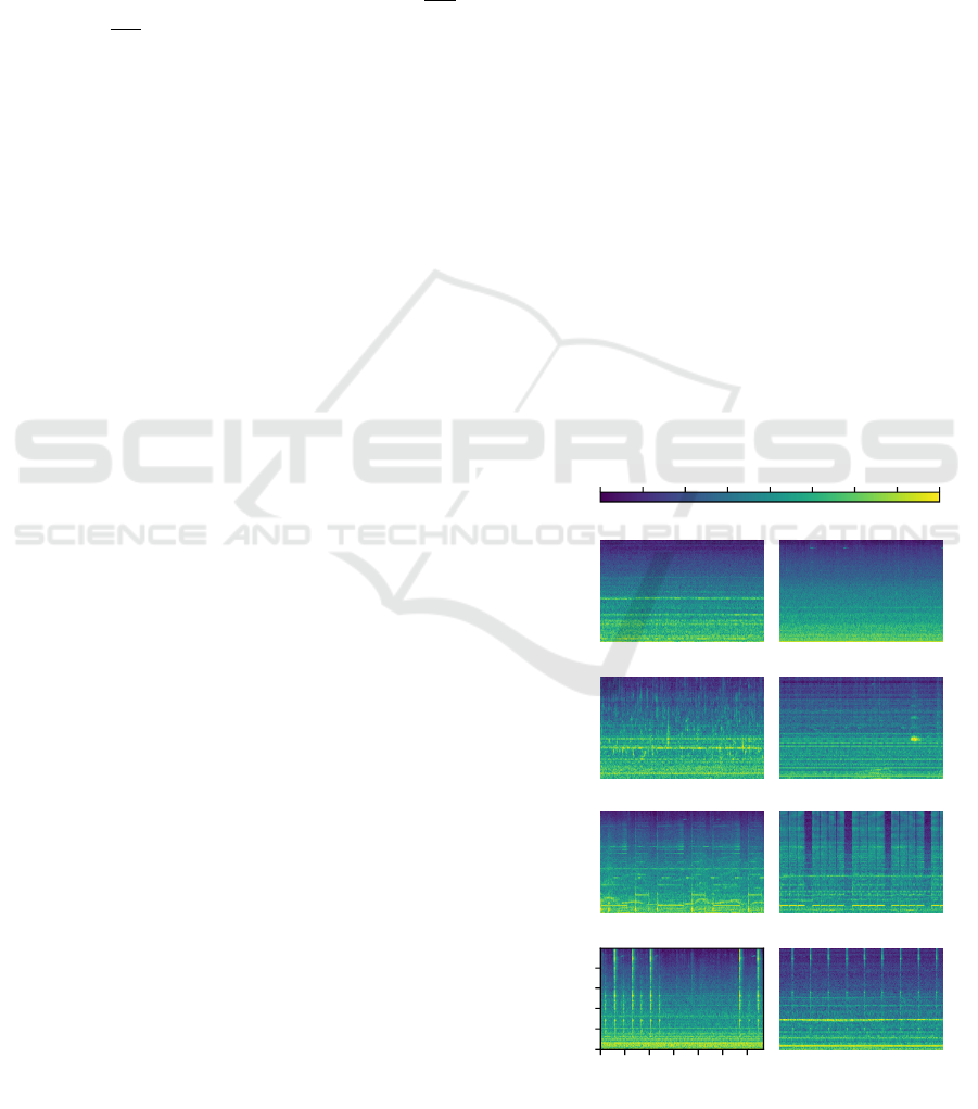
See Figure 2 for some exemplary Mel-spectrograms.

Fan normal Fan abnormal

Pump normal Pump abnormal

Slider normal Slider abnormal

0 1.5 3 4.5 6 7.5 9

Time [s]

512

1024

2048

4096

Valve normal Valve abnormal

-80 dB -70 dB -60 dB -50 dB -40 dB -30 dB -20 dB -10 dB +0 dB

Figure 2: Exemplary Mel-spectrograms of normal and ab-

normal operation with SNR= 6dB and machine id = 0.

ICAART 2021 - 13th International Conference on Agents and Artiﬁcial Intelligence

100

4.2 Feature Representations

We evaluate feature representations for ASD from

three different domains: music, images and environ-

mental sounds.

The following NNs were trained on data from an

acoustically highly similar domain to the one studied

in this work namely, environmental sounds:

VGGish. (Hershey et al., 2017)

VGGish is a vari-

ant of the VGG architecture that has successfully been

applied to image classiﬁcation. Compared to VGG16,

the number of weight layers is reduced to 11. It con-

sists of four groups of convolution+maxpooling fol-

lowed by a single 128 dimensional fully connected

layer. It was trained to classify the soundtracks of a

dataset of ≈ 70M training videos.

L3env. (Cramer et al., 2019)

Unlike the other net-

works used for feature extraction in this work that

were trained on a supervised learning task, L3 was

trained in a self-supervised manner. The audio-visual

correspondence task, i.e. predicting whether a video

frame corresponds to an audio frame, removes the

need for any external labels. Training was carried

out using ≈ 195K Videos of natural acoustic environ-

ments (e.g. human and animal sounds) extracted from

AudioSet.

Musically related tasks such as music-tagging rely

upon a rich set of features such as tone, timbre and

pitch. We assume that such features are also impor-

tant for ASD. The two NNs below were trained on

musically related tasks:

MusiCNN. (Pons and Serra, 2019)

This CNN based

architecture uses a musically motivated front-end, a

densely connected mid-end and a temporal-pooling

back-end. The shapes of the CNN ﬁlters are explicitly

designed to account for phenomena and concepts that

typically appear in music (e.g. pitch, timbre, tempo).

Since the ﬁlter dimensions on spectrograms comprise

of time and frequency, wider ﬁlters are used to ac-

count for longer temporal dependencies and higher

ﬁlters are used to capture timbral features. The Mu-

siCNN we use in this work, was trained totag mu-

sic on the MagnaTagATune dataset. Moreover, we

choose the activations from the mean-pooling layer

as feature representation.

L3music. (Cramer et al., 2019)

The only difference

to L3env is, that L3music was trained on ≈ 296K

videos of people playing musical instrument extracted

from AudioSet.

https://github.com/beasteers/VGGish

https://openl3.readthedocs.io/

https://github.com/jordipons/musicnn

https://openl3.readthedocs.io/

Lastly, the following NNs were trained on the

task of image classiﬁcation on ImageNet. The Mel-

spectrograms are converted to 224×224 images using

the Viridis colormap

as suggested by (Amiriparian

et al., 2017) in the context of snore-sound classiﬁca-

tion. Then the RGB values are standardized using the

values obtained from ImageNet. We chose images be-

cause we observed that anomalous sound patterns can

often be spotted visually in their spectral representa-

tion (M

uller et al., 2020b).

ResNet34. (He et al., 2016) ResNet uses skip-

connections to give the network the ability to bypass

blocks of convolutions. This is done to ease the van-

ishing gradient problem that would occur due to an

increased network depth. Depth allows the network to

extract a richer, more informative features. We use the

activations from the penultimate layer (right before

the 1K-way classiﬁcation head) as representation.

DenseNet121. (Huang et al., 2017) Just as ResNet,

DenseNet was designed to enable greater network

depth while being more parameter efﬁcient. Here,

the next convolutional layer receives the feature maps

from all previous layers and computes a small num-

ber of feature maps to add to the stack according to

a growth rate. This process is interleaved with 1 × 1

convolutions and average pooling to reduce the num-

ber of channels and the size of the feature maps, re-

spectively. We average-pool the activations from the

penultimate layer to receive a ﬂat feature representa-

tion.

To compare the representations above with the

more common AE-based approach we implemented

the following AE:

Autoencoder (AE). (Purohit et al., 2019) This au-

toencoder was proposed by the authors of the MIMII

dataset and serves as a strong baseline to contrast

transfer learning approaches with the more commonly

applied method of reconstruction error based anomaly

detection. Every 5 columns (time dimension) of the

Mel-spectrogram are concatenated to form a feature

vector ∈ R

320

which serves as input to a dense AE ar-

chitecture (same as (Purohit et al., 2019)). The mean

squared reconstruction error is used as loss function

and as anomaly score. The AEs are trained with a

batch size of 128 for 50 epochs, a learning rate of

0.002 and a L2 regularization of 10

−5

A brief overview of the different feature extractors

and their corresponding training domain and repre-

sentation representation size (dimensionality) is given

in Table 1.

Note that we also evaluated different color-maps but

have found the differences in the results to be neglectable.

Analysis of Feature Representations for Anomalous Sound Detection

101

4.3 Experimental Setup

To study the efﬁcacy of the different feature extrac-

tors, we propose the following workﬂow:

1. Compute the feature representations for each 10s

long sound sample in the train set with a window

size of 1s and an overlap of 0.5s. This results in

20 feature vectors per sample.

2. Apply normalization to the resulting represen-

tations and use Principal Components Analysis

(PCA) to reduce their dimensionality such that

98% of the representations variance is retained.

3. Fit a Gaussian Mixture Model (GMM) to the

transformed data.

4. At test time, obtain the transformed feature repre-

sentations for each 10s long sound sample (Steps

1 & 2) in the test set. The anomaly score for a sin-

gle transformed feature representation is given by

the weighted negative log probabilities. By mean-

pooling the scores over each sound sample, one

obtains the ﬁnal anomaly scores.

A high-level overview of this process is depicted in

Figure 1.

Model performance is measured with the Area

Under the Receiver Operating Characteristics (AUC)

which quantiﬁes how well a model can distinguish

between normal and anomalous operation across all

possible thresholds.

For each combination of machine type, machine

id, SNR and feature representation a separate GMM

is trained.

To form the test set, the same amount of normal oper-

ation data is randomly removed from the train set as

there is anomalous data, i.e. training is done on the

remaining normal operation data, anomalous data is

never seen during training and the test set is balanced.

Each experiment is repeated ﬁve times across ﬁve dif-

ferent seeds.

First, the results are conditioned on the represen-

tation, the SNR and the machine type to obtain a cor-

responding performance distributions. We use Box-

plots to report these distributions grouped by the do-

main of the representations. The results for image,

music and environmental sound based representations

are depicted in Figure 4, Figure 5 and Figure 6, re-

spectively. Then we select the best performing (fea-

ture extractor - machine type) pairs and compare the

results by domain as well as with the autoencoder

baseline in Figure 7.

In Table 2 we additionally condition the results

from Figure 7 on the machine id to gain more insights

on how the models perform on each individual ma-

Table 1: Overview of the different feature extractors.

Name Trained on Rep. size

L3env Environmental

sounds

512

VGGish 128

ResNet34

Images

512

DenseNet121 1024

MusiCNN

Music

753

L3music 512

chine id. Each cell represents the average AUC ± one

standard deviation.

A detailed discussion of the results follows in Sec-

tion 5.

4.4 Choice of Hyperparameters

The crucial hyperparameters of GMMs are the num-

ber of mixtures and the covariance matrix type. To

determine suitable hyperparameters, we randomly se-

lected three feature extractors and two machine types

with SNR= 0dB and ID= 0. Then we computed the

average AUC with a varying number of mixture com-

ponents {1,4, 8,. .. 28} with full and diagonal covari-

ance matrices (Figure 3).

While the features extracted from MusiCNN ap-

pear to be stable with respect to the number of mix-

tures and the covariance type, results for other rep-

resentations quickly decline when using full covari-

ance matrices and an increasing number of mixtures.

Hence, the GMM becomes too expressive. This ef-

fect is not observed when using diagonal covariance

matrices as the results are stable and slightly increase

with the number of mixtures.

Since anomalous data is usually scarce, it is not

feasible to tune the hyperparameters on every setting

and consequently a stable set of hyperparameters is

desirable. Therefore, we use a GMM with 20 mixture

components and diagonal covariance matrices for all

experiments in this work.

5 RESULTS

In this section we ﬁrst discuss the results for each in-

dividual feature extractor domain. Then we present

ﬁndings that apply to all domains. Finally, we discuss

the limitations of our analysis.

5.1 Image based Representations

DenseNet121 outperforms ResNet34 in terms of the

mean and median AUC on all machine types except

ICAART 2021 - 13th International Conference on Agents and Artiﬁcial Intelligence

102

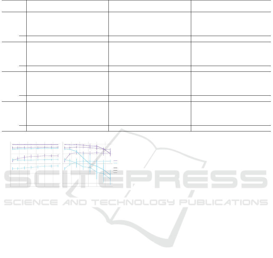
Table 2: Mean AUCs for all experiments.

SNR -6dB 0dB 6dB

Machine ID AE Env. Imgs. Music AE Env. Imgs. Music AE Env. Imgs. Music

Fan

0 53.0±1.6 58.7±1.2 57.3±1.3 61.4±1.0 58.0±3.5 67.0±0.8 62.7±0.8 71.6±0.4 74.5±1.7 83.7±1.3 74.1±0.8 88.5±0.6

2 68.7±1.6 70.9±1.1 58.5±1.7 66.6±1.7 85.9±1.5 85.1±0.6 69.7±0.9 82.9±0.9 93.0±1.3 92.8±0.5 81.4±0.5 96.4±0.5

4 56.8±1.2 56.3±1.8 52.0±1.1 52.8±1.5 76.5±2.1 76.5±0.7 65.9±1.4 79.6±1.4 91.5±1.2 93.5±0.6 85.9±1.1 98.9±0.7

6 78.9±2.1 87.4±0.6 87.8±1.0 94.8±1.0 93.9±0.8 94.7±0.2 97.7±0.1 99.9±0.1 98.7±0.3 98.4±0.2 99.4±0.1 100.0±0

∅ 64.4±10.4 68.3±12.7 63.9±14.4 68.9±16.2 78.6±13.7 80.8±10.5 74.0±14.3 83.5±10.6 89.4±9.2 92.1±5.5 85.2±9.5 95.9±4.6

Pump

0 71.4±2.8 78.6±1.5 75.8±2.1 84.0±1.5 72.5±1.7 87.9±1.2 85.1±1.1 85.4±0.4 87.1±1.0 96.0±0.5 94.5±0.6 94.1±0.4

2 53.2±3.0 55.4±1.1 68.1±2.1 62.3±1.3 55.1±2.4 65.9±2.5 90.4±1.3 77.8±2.0 60.1±1.5 74.3±1.2 97.6±0.4 81.6±0.9

4 93.0±2.3 96.1±1.3 86.5±1.1 76.2±2.4 99.6±0.6 99.5±0.3 96.7±1.1 88.3±1.6 100.0±0 100.0±0. 99.8±0.1 98.9±1.0

6 71.8±3.0 61.6±3.2 58.7±3.8 67.2±2.6 88.1±2.6 83.1±1.8 79.9±2.4 86.0±0.7 97.8±1.0 97.9±0.3 96.4±1.6 98.7±0.1

∅ 72.4±14.5 72.9±16.4 72.3±10.7 72.4±8.8 78.8±17.0 84.1±12.5 88.0±6.5 84.4±4.2 86.2±16.1 92.0±10.6 97.1±2.2 93.3±7.2

Slider

0 91.5±1.9 98.5±0.3 99.5±0.3 99.1±0.3 96.4±0.8 99.8±0.1 99.9±0.1 99.9±0.1 99.2±0.3 100.0±0 100.0±0 100.0±0

2 77.9±1.6 83.0±0.9 91.7±1.0 83.2±1.0 86.5±0.6 93.1±0.8 97.0±0.5 92.7±0.6 94.4±0.8 99.0±0.3 99.5±0.2 98.9±0.2

4 71.0±2.7 82.0±1.4 70.6±2.3 79.2±1.7 88.9±3.0 95.6±0.7 84.0±1.0 94.4±0.8 95.6±1.8 98.8±0.3 92.4±0.5 98.6±0.4

6 55.3±2.8 66.8±2.4 56.8±3.8 69.8±1.8 61.8±3.1 87.3±2.8 63.3±3.1 86.7±2.2 71.7±4.6 95.9±1.3 74.9±4.4 96.4±0.9

∅ 73.9±13.4 82.6±11.6 79.7±17.5 82.8±10.9 83.4±13.3 93.9±4.8 86.1±14.9 93.5±5.0 90.2±11.3 98.4±1.7 91.7±10.6 98.5±1.4

Valve

0 50.3±4.7 61.0±1.7 73.4±1.7 70.3±2.2 51.4±2.4 75.4±3.6 88.6±1.7 78.1±2.9 60.5±8.7 74.2±0.7 90.5±1.7 75.2±1.2

2 62.0±3.5 74.9±1.9 63.9±3.0 70.3±2.4 72.2±2.9 82.0±2.1 70.8±1.7 80.2±1.6 75.0±6.0 85.0±1.0 72.6±1.5 86.3±0.8

4 61.5±3.0 64.8±3.3 64.2±2.0 68.2±1.7 65.6±4.2 74.6±1.9 70.8±2.7 79.6±2.6 66.9±3.4 82.4±1.8 85.4±2.5 84.2±0.8

6 51.2±2.9 55.8±2.6 59.4±3.3 58.7±2.9 57.5±2.0 57.8±3.6 55.9±1.7 60.7±2.6 66.3±5.0 72.0±0.8 66.0±2.1 74.2±1.1

∅ 56.2±6.6 64.2±7.5 65.2±5.8 66.9±5.4 61.7±8.5 72.5±9.6 71.5±12.0 74.7±8.6 67.2±7.8 78.4±5.7 78.6±10.2 80.0±5.5

0 5 10 15 20 25

Mixture Components

100

AUC

Covariance = diag

0 5 10 15 20 25

Mixture Components

Covariance = full

Machine

Pump

Slider

Setting

L3env

DenseNet121

MusiCNN

Figure 3: Small scale study to determine the GMM hyper-

parameters.

for slider where the difference is insigniﬁcant. More-

over, there are no major differences with respect to the

variance. The most striking performance differences

are observed on pump and valve.

A possible explanation for the superiority of

DenseNet121 is that it also outperforms ResNet34 in

terms of classiﬁcation accuracy on ImageNet by ex-

tracting a richer, more nuanced and more discrimina-

tive set of features and that this superiority also carries

over to our setting.

Recent work (M

uller et al., 2020b) did not evalu-

ate their method on DenseNet based representations

and concluded that ResNet based features are best

suited for anomalous sound detection. In contrast,

here we have found that in our setting, ResNet is out-

performed by DenseNet. Our results indicate that fur-

ther studies are necessary to explore the space of im-

age based feature extractors for ASD.

5.2 Music based Representations

From Figure 5 we can observe that L3music shows

signiﬁcantly better results on slider and valve than

MusiCNN. On the other hand, MusiCNN outperforms

L3music on fan and pump.

While fan and pump have a stationary sound pat-

tern, slider and valve exhibit non-stationary patterns.

Our interpretation is that MusiCNN’s rectangular hor-

izontal ﬁlters (time dimension) are especially well

suited to extract features that describe the normal op-

eration of stationary sounds since they are almost con-

stant and vary only slightly over time. Then, anoma-

lies will be characterized by the absence of certain

features for example because the machine randomly

stops operating, suddenly exhibits irregular sounds

or the pitch of the sound changes due to damages.

For slider and valve, MusiCNN’s music tagging task

might be too restrictive compared to the very general

audio-visual correspondence task of L3music.

5.3 Environmental Sound based

Representations

From the inspection of Figure 6 we can conclude that

L3env yields far better results on slider and valve

compared to VGGish. On fan and pump, both feature

extractors perform on-par.

Just as in Section 5.2, the most obvious perfor-

mance differences can be observed on non-stationary

machine sounds. We noticed that on slider and valve,

the VGGish feature representations are highly redun-

dant. That is, PCA reduces representations down to

Analysis of Feature Representations for Anomalous Sound Detection

103

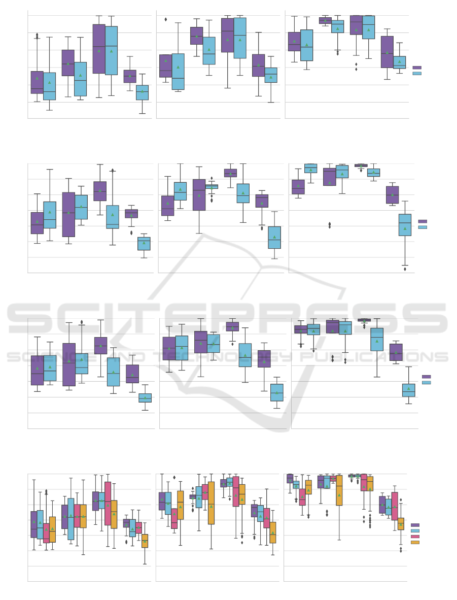
Fan Pump Slider Valve

Machine

100

AUC

SNR = -6dB

Fan Pump Slider Valve

Machine

SNR = 0dB

Fan Pump Slider Valve

Machine

SNR = 6dB

Representation

DenseNet121

ResNet34

Figure 4: Comparison between image based representations.

Fan Pump Slider Valve

Machine

100

AUC

SNR = -6dB

Fan Pump Slider Valve

Machine

SNR = 0dB

Fan Pump Slider Valve

Machine

SNR = 6dB

Representation

L3music

MusiCNN

Figure 5: Comparison between music based representations.

Fan Pump Slider Valve

Machine

100

AUC

SNR = -6dB

Fan Pump Slider Valve

Machine

SNR = 0dB

Fan Pump Slider Valve

Machine

SNR = 6dB

Representation

L3env

VGGish

Figure 6: Comparison between environmental sound based representations.

Fan Pump Slider Valve

Machine

100

AUC

SNR = -6dB

Fan Pump Slider Valve

Machine

SNR = 0dB

Fan Pump Slider Valve

Machine

SNR = 6dB

Category

Music

Environmental

Images

Figure 7: Comparison between the best performing representations and the autoencoder baseline. Music representations:

MusiCNN for Fan and Pump, L3music for Slider and Valve. Environmental Sounds: L3env. Images: DenseNet121.

ICAART 2021 - 13th International Conference on Agents and Artiﬁcial Intelligence

104

a very small number of features. Essentially, VG-

Gish extracts very similar features for all recordings

thereby hindering the creation of an informative nor-

mal operation model.

Previous work (Cramer et al., 2019) used L3 rep-

resentations for sound event detection and reports su-

perior performance compared to VGGish. In our case

these results also hold for ASD. Moreover, we con-

juncture that the self-supervised audio-visual corre-

spondence task extracts a richer set of features as it

is a more complex task that needs more expressive,

general purpose features compared to VGGish’s more

narrow classiﬁcation objective.

5.4 General Observations

Generally, the introduction of background noise con-

siderably reduces the performance of all representa-

tions. Moreover, all representations are affected by

background noise in the same way i.e. noise does not

change the performance ranking.

Fan is the machine type that suffers the most from

increased background noise. This is because fan

sounds and background noise exhibit a similar sound

pattern, making them harder to distinguish.

We found the valve machine type samples (highly

non-stationary) to be the hardest to detect anomalous

operations on, and slider to be the easiest (clearly vis-

ible anomalies in the Mel-spectrograms).

When averaged over the machine id (Table 2), all

transfer learning approaches outperform the AE base-

line. Thus, this conﬁrms our hypothesis that transfer-

ring knowledge from pretrained NNs increases ASD

performance.

Music based representations achieve the best re-

sults with 8/12 top performances. Both image and en-

vironmental sound based representations account for

2/12 top performances, each.

These results challenge the intuition that closely

matching the domain results in better downstream

task performance as one might have suspected envi-

ronmental sound based representations to yield the

best results because they have the smallest domain

mismatch with machine sounds. However, it might be

more important to use audio content that maximizes

the discriminative power of the representations, inde-

pendently of the downstream domain (Cramer et al.,

2019). In the case of L3 based representations, peo-

ple playing musical instruments have a greater degree

of audio visual correspondence than environmental

videos. Moreover, music itself provides a richer, more

diverse training signal than environmental sounds.

5.5 Limitations of the Analysis

Evaluating the different representations presents a

challenge as it is hard to ﬁnd the particular reasons

why one representation works better than another

since the feature extractors were trained on different

dataset with a varying amount of data. Additionally,

they all use different (black-box) neural network ar-

chitectures and slightly different Mel-spectrogram pa-

rameters. Moreover, their domain varies, the train-

ing task was either supervised or self-supervised and

no information on the speciﬁc type of anomaly of a

recording is provided by the MIMII dataset.

6 CONCLUSION

In this work, we evaluated the effectiveness of trans-

ferring knowledge from pretrained NNs for anoma-

lous sound detection using the feature extraction

paradigm. Our approach was evaluated with feature

representations from the image, environmental sound

and music domain and allows for fast experimentation

as only shallow models have to be trained. We showed

that almost all representations yield competitive ASD

performance with an advantage for music based rep-

resentations. Thus, we have found that even under

a domain mismatch between the feature extractor and

the downstream ASD task, the studied representations

are suitable for ASD. This suggests that pretraining on

a closely related domain might not always be neces-

sary which results in a greater ﬂexibility in the choice

of pretraining strategies and datasets. The key ﬁnding

of this work is that a relatively simple experimental

setup based on transfer learning can yield compet-

itive ASD performance without the need to develop

a completely new model. Hence, we argue that fu-

ture approaches should compare themselves against

transfer learning approaches. Furthermore, this work

provides guidance on the choice of feature extractors

for future ASD research. In future work, one might

experiment with the best feature extractors from this

work in conjunction with a sequence-to-sequence au-

toencoder. This approach would explicitly account

for the temporal structure of sound and might could

performance on machine types with a non-stationary

sound proﬁle.

REFERENCES

Amiriparian, S., Gerczuk, M., Ottl, S., Cummins, N., Fre-

itag, M., Pugachevskiy, S., Baird, A., and Schuller,

Analysis of Feature Representations for Anomalous Sound Detection

105

B. W. (2017). Snore sound classiﬁcation using image-

based deep spectrum features. In INTERSPEECH,

volume 434, pages 3512–3516.

Bayram, B., Duman, T. B., and Ince, G. (2020). Real time

detection of acoustic anomalies in industrial processes

using sequential autoencoders. Expert Systems, page

e12564.

Beckmann, P., Kegler, M., Saltini, H., and Cernak, M.

(2019). Speech-vgg: A deep feature extractor for

speech processing. arXiv preprint arXiv:1910.09909.

Chi, P.-H., Chung, P.-H., Wu, T.-H., Hsieh, C.-C., Li, S.-

W., and Lee, H.-y. (2020). Audio albert: A lite bert

for self-supervised learning of audio representation.

arXiv preprint arXiv:2005.08575.

Cramer, J., Wu, H.-H., Salamon, J., and Bello, J. P. (2019).

Look, listen, and learn more: Design choices for

deep audio embeddings. In IEEE International Con-

ference on Acoustics, Speech and Signal Processing

(ICASSP), pages 3852–3856. IEEE.

Devlin, J., Chang, M.-W., Lee, K., and Toutanova, K.

(2019). Bert: Pre-training of deep bidirectional trans-

formers for language understanding. In Proceedings

of the 2019 Conference of the North American Chap-

ter of the Association for Computational Linguistics,

pages 4171–4186.

Donahue, J., Jia, Y., Vinyals, O., Hoffman, J., Zhang, N.,

Tzeng, E., and Darrell, T. (2014). Decaf: A deep con-

volutional activation feature for generic visual recog-

nition. In International conference on machine learn-

ing, pages 647–655.

Duman, T. B., Bayram, B., and

Ince, G. (2019). Acoustic

anomaly detection using convolutional autoencoders

in industrial processes. In International Workshop on

Soft Computing Models in Industrial and Environmen-

tal Applications, pages 432–442. Springer.

Hasan, M. A., Abu-Bakar, M.-H., Razuwan, R., and Nazri,

Z. (2018). Deep neural network tool chatter model

for aluminum surface milling using acoustic emmi-

sion sensor. In MATEC Web of Conferences.

Hayashi, T., Komatsu, T., Kondo, R., Toda, T., and Takeda,

K. (2018). Anomalous sound event detection based on

wavenet. In 2018 26th European Signal Processing

Conference (EUSIPCO), pages 2494–2498. IEEE.

He, K., Zhang, X., Ren, S., and Sun, J. (2016). Deep resid-

ual learning for image recognition. In Proceedings of

the IEEE conference on computer vision and pattern

recognition, pages 770–778.

Hershey, S., Chaudhuri, S., Ellis, D. P., Gemmeke, J. F.,

Jansen, A., Moore, R. C., Plakal, M., Platt, D.,

Saurous, R. A., Seybold, B., et al. (2017). Cnn archi-

tectures for large-scale audio classiﬁcation. In IEEE

International Conference on Acoustics, Speech and

Signal Processing (ICASSP), pages 131–135. IEEE.

Huang, G., Liu, Z., Van Der Maaten, L., and Weinberger,

K. Q. (2017). Densely connected convolutional net-

works. In Proceedings of the IEEE conference on

computer vision and pattern recognition, pages 4700–

4708.

Kawaguchi, Y., Tanabe, R., Endo, T., Ichige, K., and

Hamada, K. (2019). Anomaly detection based on an

ensemble of dereverberation and anomalous sound ex-

traction. In IEEE International Conference on Acous-

tics, Speech and Signal Processing (ICASSP), pages

865–869.

Koizumi, Y., Murata, S., Harada, N., Saito, S., and Ue-

matsu, H. (2019). Sniper: Few-shot learning for

anomaly detection to minimize false-negative rate

with ensured true-positive rate. In IEEE International

Conference on Acoustics, Speech and Signal Process-

ing (ICASSP), pages 915–919. IEEE.

Koizumi, Y., Saito, S., Uematsu, H., and Harada, N. (2017).

Optimizing acoustic feature extractor for anomalous

sound detection based on neyman-pearson lemma. In

2017 25th European Signal Processing Conference

(EUSIPCO), pages 698–702. IEEE.

Marchi, E., Vesperini, F., Eyben, F., Squartini, S., and

Schuller, B. (2015). A novel approach for automatic

acoustic novelty detection using a denoising autoen-

coder with bidirectional lstm neural networks. In

IEEE international conference on acoustics, speech

and signal processing (ICASSP), pages 1996–2000.

IEEE.

uller, R., Illium, S., , Ritz, F., Schr

oder, T., Platschek, C.,

Ochs, J., and Linnhoff-Popien, C. (2020a). Acoustic

leak detection in water networks. Technical report.

uller, R., Ritz, F., Illium, S., and Linnhoff-Popien, C.

(2020b). Acoustic anomaly detection for machine

sounds based on image transfer learning. arXiv

preprint arXiv:2006.03429.

Oord, A. v. d., Dieleman, S., Zen, H., Simonyan, K.,

Vinyals, O., Graves, A., Kalchbrenner, N., Senior,

A., and Kavukcuoglu, K. (2016). Wavenet: A

generative model for raw audio. arXiv preprint

arXiv:1609.03499.

Peters, M. E., Neumann, M., Iyyer, M., Gardner, M., Clark,

C., Lee, K., and Zettlemoyer, L. (2018). Deep con-

textualized word representations. In Proceedings of

NAACL-HLT, pages 2227–2237.

Pons, J. and Serra, X. (2019). musicnn: Pre-trained con-

volutional neural networks for music audio tagging.

arXiv preprint arXiv:1909.06654.

Purohit, H., Tanabe, R., Ichige, K., Endo, T., Nikaido,

Y., Suefusa, K., and Kawaguchi, Y. (2019). Mimii

dataset: Sound dataset for malfunctioning industrial

machine investigation and inspection. arXiv preprint

arXiv:1909.09347.

Ruder, S. (2018). NLP’s ImageNet moment has arrived.

Rushe, E. and Namee, B. M. (2019). Anomaly detection

in raw audio using deep autoregressive networks. In

IEEE International Conference on Acoustics, Speech

and Signal Processing (ICASSP), pages 3597–3601.

Suefusa, K., Nishida, T., Purohit, H., Tanabe, R., Endo, T.,

and Kawaguchi, Y. (2020). Anomalous sound detec-

tion based on interpolation deep neural network. In

IEEE International Conference on Acoustics, Speech

and Signal Processing (ICASSP), pages 271–275.

ICAART 2021 - 13th International Conference on Agents and Artiﬁcial Intelligence

106