
Robustness-driven Exploration with Probabilistic Metric Temporal
Logic
Xiaotian Liu
1
, Pengyi Shi
1
, Tongtong Liu
1
, Sarra Alqahtani
1
, Paul Pauca
1
and Miles Silman
2
1
Computer Science Department, Wake Forest University, Winston Salem, NC, U.S.A
2
Biology Department, Wake Forest University, Winston Salem, NC, U.S.A.
Keywords: Exploration, Metric Temporal Logic, Robustness, MCMC.
Abstract: The ability to perform autonomous exploration is essential for unmanned aerial vehicles (UAV) operating in
unknown environments where it is difficult to describe the environment beforehand. Algorithms for
autonomous exploration often focus on optimizing time and full coverage in a greedy fashion. These
algorithms can collect irrelevant data and wastes time navigating areas with no important information. In this
paper, we aim to improve the efficiency of exploration by maximizing the probability of detecting valuable
information. The proposed approach relies on a theory of robustness based on Probabilistic Metric Temporal
Logic (P-MTL) which is traditionally applied to offline verification and online control of hybrid systems. The
robustness values would guide the UAV towards areas with more significant information by maximizing the
satisfaction of the predefined P-MTL specifications. Markov Chain Monte Carlo (MCMC) is utilized to solve
the P-MTL constraints. We tested our approach over Amazonian rainforest to detect areas occupied by illegal
Artisanal Small-scale Gold Mining (ASGM) activities. The results show that our approach outperforms a
greedy exploration approach from the literature by 38% in terms of ASGM coverage.
1 INTRODUCTION
Exploration is often an important first step in tasks of
robotics and autonomous vehicles, such as mapping,
rescue missions, or path planning in unknown
environments. Techniques that tackle this problem
typically focus on exploration time and coverage, i.e.
how fast and how much of an unexplored area can be
explored (Bircher et al., 2016; Yamauchi, 1997; Selin
et al., 2019). Although optimizing coverage and time
for exploration problems is crucial, it is important in
some problem domains to consider exploiting the
detected information about the environment while
exploring it to prioritizing the exploration of
interesting areas encountered during flight. Adding
such spatial and temporal considerations into
exploration enhances the decision robustness about
the navigation behaviour of the UAV and introduces
some predictability on where the vehicle could move
next. Moreover, it is usually more desirable to gather
knowledge and information about certain areas than
wasting the vehicle’s resources such as flight time or
its local storage exploring the whole environment.
In this paper, we address the problem of mapping
mercury-based Small-scale Gold Mining (ASGM) in
Amazonian Forest (Koymans, 1990). Mercurybased
ASGM causes more mercury pollution than any other
human activity on Earth, leading to major effects on
the environment, health, and local economies. It is a
global issue affecting 10 to 19 million people in over
70 countries (Adler et al., 2014). Though satellite
remote sensing would be ideal for monitoring ASGM
sites (e.g. (Heng et al., 2015)), satellites do not
currently produce images of sufficient resolution to
accurately detect ASGM and differentiate, for
example, between active and inactive mining sites
(e.g. (González-Baños and Latombe, 2002)).
Moreover, satellite monitoring is not possible in
cloudy and rainy weather which is very common in
areas like the Amazon forest. UAVs can overcome
those issues. They are affordable, easy to use,
versatile, and even suitable in barely accessible areas.
They also deliver high resolution data, mostly
independent of cloud cover condition. However, the
UAV field of view is significantly smaller than that
of a satellite. To use UAVs to collect information in
Amazon, its acquisition of image data needs to reduce
the flight time, the required storage, and classification
burden of the collected images. According to
researchers who collect images using a small UAV in
Liu, X., Shi, P., Liu, T., Alqahtani, S., Pauca, P. and Silman, M.
Robustness-driven Exploration with Probabilistic Metric Temporal Logic.
DOI: 10.5220/0010192100570066
In Proceedings of the 13th International Conference on Agents and Artificial Intelligence (ICAART 2021) - Volume 2, pages 57-66
ISBN: 978-989-758-484-8
Copyright
c
2021 by SCITEPRESS – Science and Technology Publications, Lda. All rights reserved
57

Amazon Forest for their ASGM research (Karaman
and Frazzoli, 2019), a full exploration of a small area
as of 8x8 km2 requires almost 8 separate flights; each
flight has been done in 4 hours; acquiring 7200
images.
In this specific instance of exploration problem,
the UAV would explore the given simulated map
looking for ASGM. The environment is unknown and
the only input to the system is the onboard recognition
system for materials and machinery used in ASGM.
The goal is to improve the efficiency of exploration:
i.e. to maximize the probability of detecting ASGM
relative to the exploration effort that has been
expended. To achieve that, we develop a novel
robustness-driven exploration (RDE) approach to
constrain a UAV movement according to user-
defined spatial and temporal constraints expressed in
P-MTL. These constraints guide the exploration into
ASGM areas in the environment which we call Areas
of Interest (AoI) based on the online detection of
ASGM features. The first contribution of our work is
the proposal of a method to explore unknown
environment according to a robustness function that
considers the degree of satisfaction of P-MTL
specifications of AoI. By utilizing the notion of
robustness for Metric Temporal Logic (MTL)
(Karaman and Frazzoli, 2011), we can quantify how
robustly a UAV’s exploration decision satisfies a P-
MTL specification.
The second contribution is adopting MCMC to
solve the P-MTL constraints. The MCMC technique
is used as a local exploration strategy and is combined
with a simplified version of Frontier Exploration
(Yamauchi, 1997) for global exploration. When a
new AoI is available close to the UAV, the local
exploration strategy is used, but when it is far away
from any AoI, previously seen but not-visited-yet
positions with potential high robustness are explored
instead. This simple technique helps the MCMC
avoid getting stuck locally when exploring large areas
with small or zero robustness values (i.e. no ASGM).
The performance of RDE is evaluated by
simulating UAV exploration over five different
regions of the Amazon Forest in Peru to detect areas
occupied by illegal mining activities. We test RDE
against the Autonomous Exploration Planner (AEP)
proposed in (Selin et al., 2019). The results show that
our proposed approach outperforms AEP in terms of
AoI coverage by 38%.
The remainder of this paper is organized as
follows. The next section further discusses the related
work of the autonomous exploration and the temporal
logic robustness and its application to exploration and
navigation problems. In section 3, we introduce the
problem definition and briefly review MTL
robustness and P-MTL. Section 4 discusses the
proposed approach, and Section 5 presents the results
and discusses future work.
2 RELATED WORK
Early autonomous exploration methods explored
simple environments, for example, by following walls
or similar obstacles. Frontier exploration (Yamauchi,
1997) was the first exploration method that could
explore a generic 2D environment. It defines frontier
regions as the borders between free and unexplored
areas. Exploration is done by sequentially navigating
close frontiers. Repetition of this process leads to
exploring the whole space. Advanced variants of this
algorithm were presented in (Alqahtani et al., 2018;
Ayala et al., 2013; Vasile et al., 2017) also improving
the coverage of unknown space along the path to the
frontier.
Next-best-view (NBV) exploration is a common
alternative to frontier-based exploration. A Receding
Horizon NBV planner is developed in (Bircher et al.,
2016), for online autonomous exploration of
unknown 3D spaces. The proposed planner employed
the rapidly exploring random tree RRT with a cost
function that considers the information gain at each
node of the tree. A path to the best node was extracted
and the algorithm was repeated after each time the
vehicle moved along the first edge of the best path.
An extension of this work is proposed in (Selin et al.,
2019) to resolve the problem of getting stuck in local
minima by extending it with frontier-based planner
for global exploration. Our approach also samples
NBV according to the current vision of the UAV. In
contrast to previously mentioned research, the views
are randomly sampled as potential targets in our
approach via MCMC and evaluated by their
robustness values of the P-MTL constraints. In most
cases, very few sampled positions suffice to
determine a reasonably good next target.
Recently, temporal logics have been used in the
context of robotic motion and path planning in
unknown environments. For instance, deterministic
μ-calculus was used to define specifications for
sampling-based algorithms (Barbosa et al., 2019),
Linear Temporal Logic (LTL) was coupled with
RRT* (Caballero et al., 2018), robustness of Metric
Temporal Logic (MTL) has been embedded in A*
(Esdaile and Chalker, 2018) to increase the safety of
UAVs navigating adversarial environments. Ayala et
al. assumed that some properties of unknown
environments can be identified earlier and used in
ICAART 2021 - 13th International Conference on Agents and Artificial Intelligence
58
Linear Temporal Logic (LTL) formulas, such that the
exploration terminates once the formula is satisfied
(Swenson et al., 2011). In (Asner, 2013), the
researchers use co-safe LTL (cs-LTL) in their motion
planning algorithm to compromise between
satisfaction of customer demands and violation of
road rules).
3 PRELIMINARIES
In this section, we provide the syntax and semantics
for MTL and P-MTL specifications and how we use
them to formally define our exploration problem.
3.1 MTL Robustness
Definition 1: (MTL Syntax). Let AP be the set of
atomic propositions and be a time interval of . The
MTL formula is recursively defined using the
following grammar (Karaman and Frazzoli, 2011):
(1)
T is the Boolean True, , ¬ is the Boolean
negation, and are the logical OR and AND
operators, respectively.
is the timed until operator
and the interval I imposes timing constraints on the
operator. Informally,
means that
must hold
until
holds, which must happen within the interval
I. The implication (), Always (□), Next (○), and
Eventually (◊) operators can be derived using the
above operators.
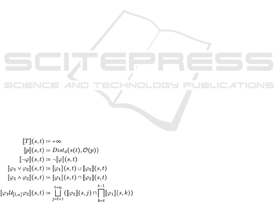
To formally measure the robustness degree of at
the trajectory position at time , the robustness
semantics of is recursively defined as taken directly
from (Dokhanchi et al., 2014):
where stands for maximum, stands for minimum,
,and . The robustness is a real-valued
function of the trajectory position s with the following
important property stated in Theorem 1.
Theorem 1 (Dokhanchi et al., 2014): For any
and MTL formula , if is negative, then
does not satisfy the specification at time . If it is
positive, then satisfies at . If the result is zero,
then the satisfaction is undefined.
MTL robustness is adopted in this research to
measure how robust the exploration decision of the
UAV at any point of time with respect to its
specification expressed in MTL (Dokhanchi et al.,
2014). If an MTL specification valuates to positive
robustness , then the decision is right and, moreover,
can tolerate perturbations up to and still satisfy the
specification. Similarly, if is negative, then the
decision does not satisfy with a violation equal to -
.
3.2 P-MTL
Probabilistic-MTL (P-MTL) (Fainekos and Pappas,
2006) is an extension of MTL supporting reasoning
over both stochastic states and stochastic predictions
of states. The predictive operator is used to
refer to observed, estimated, and predicted states. The
predictive operator is informally defined as follows:
Observed state value:
Estimated state value:
Predicted state value:
where is the observation time, is the prediction
time, and is the stochastic state under investigation.
The value of
is the observed value of state at
time . On the other hand,
is the estimated value
of state s at time which is the prediction made at
time about the value of s at time . This operator is
useful when the detection results are in form of
probability distribution. The value of
is a
prediction made at time about the value of state s at
time
′
.
′
may be larger than (prediction about
the future) or smaller than (prediction about the
past).
4 AUTONOMOUS
EXPLORATION WITH P-MTL
ROBUSTNESS
The question we address in this work is: starting with
partially known map, which decisions should the
UAV perform to explore
completely and as fast
as possible guided by the detection results of ASGM?
Problem (P-MTL Satisfaction). For an P-MTL
specification , the P-MTL satisfaction problem
consists of finding an output state of the system
starting from some initial state
under a control
Robustness-driven Exploration with Probabilistic Metric Temporal Logic
59
input signal such that does satisfy the
specification with the required robustness .
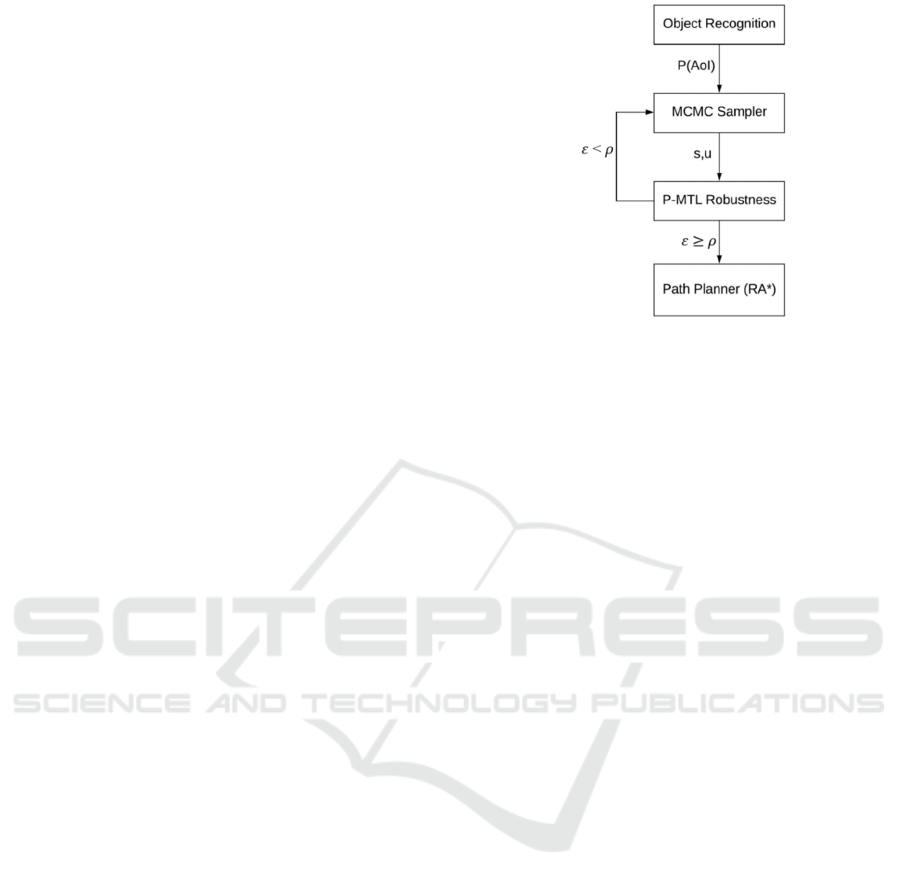
An overview of our proposed approach to resolve
Problem (P-MTL Satisfaction) is shown in Fig.1. At
every time step, the object recognition module would
generate probabilities for the detected AoI inside the
UAV’s vision. Then, based on the detection results,
MCMC sampler would select a position from the set
of neighbors and a vector of parameters that
characterize the control input signal (i.e. speed and
altitude). The selected position is then analyzed by the
P-MTL robustness analyzer which would return a
robustness score . In turn, if is less than a
predefined threshold then the stochastic sampler
would be called again to select another position for
analysis. If in this process, a position with greater
than is found, it is used by the path planner RA*
(Esdaile and Chalker, 2018) to move the UAV to that
position. RA* has been originally implemented to
embed MTL robustness into A* to avoid mobile
obstacles in hostile environments. We change its
MTL constraints to allow the UAV to explore the AoI
available around the path while still be target
oriented.
Using the MTL syntax (Definition 1) and the
informal definition of P-MTL, we define the P-MTL
specification of our problem of RDE as follows:
(2)
The first property of the formula
represents a safety constraint requiring the UAV to
keep its battery level above a certain threshold
to get back to homebase. The threshold
would
be updated dynamically based on the current position
of the UAV in the map.
specifies that the UAV should stay inside areas with
a likelihood of being AoI above . This property is
classified as a liveness (i.e. preferred) property.
To decrease the possibility that the UAV wastes
time exploring non-AoI, the conditional liveness
property
asks the UAV to stay a
maximum of time steps inside areas with likelihood
of being less than and when that happened the
UAV must immediately (i.e. next decision) find
another area with higher estimation of AoI or
terminate the mission and go back to homebase.
Figure 1: Proposed approach for RDE problem.
In order to compute the P-MTL robustness for our
exploration problem, we must define the Signed
Distance,
to reflect the domain properties
(Dokhanchi et al., 2014). In this paper, we define two
functions to measure the distance from the
propositions of the AoI and the minimum battery
level Bmin (Fig.2). The location pins symbol
represents AoI and the quadrotor drone symbol is the
exploring UAV. The proposed approach analyzes the
neighbor positions of the current position of the
UAV and makes a decision about the next target
based on the distance and depth functions given in
Definition 2 and 3 next.
Definition 2 (AoI function): Given that
is
the position that is under robustness analysis, is the
probability of
being inside an AoI given by the
object recognition system, and is the minimum
threshold for the detection results, the
between
and the closest AoI is defined as:
) =
(3)
Then, we define a depth function to measure the
distance between the position
that is under
robustness analysis and the UAV resource limit.
We assume that the UAV starts its mission with full
battery (B=100%) to explore the assigned
environment. Given that the UAV moves with
velocity, we define a region centered at with
radius
to find the farthest positions that the
UAV could travel while still being able to go back
home.
With this region defined (Fig. 2), we can define
the function
.
ICAART 2021 - 13th International Conference on Agents and Artificial Intelligence
60

Figure 2: The structure of the Signed Distance in RDE
domain.
Definition 3 (Battery Life function): Given
that B is the current level of the battery life and
is the battery minimum threshold,
function for the UAV at position
is
defined as:
(4)
The function
measures the distance
to the closest edge of the region defined by a
constraint centered on the position
. It should be
noted that the defined regions include a third
dimension for time. Therefore, the outer edges of the
structure shown in Fig.2 would shrink over time.
Given a position
, we have defined a robustness
metric
that denotes how
robustly
satisfies (or falsifies) at time t. The
robustness metric
maps each position
to a real
number . The sign of indicates whether
satisfies
and its magnitude || measures its robustness value.
More generally, given a robustness threshold
and a neighboring function to return a set of
positions which are in neighboring distance (i.e.
within the range of the UAV) from the UAV’s current
location, we need to find:
(5)
Using the dist and depth functions, the P-MTL
robustness degree of in equation 2 can be point-
wise computed for each position
under robustness
analysis to solve the RDE problem in equation 5.
The robustness of the safety property in equation
2 measured at each neighbor position since it must
hold during the whole trajectory. To measure the
robustness of the safety constraint for position s, we
use the MTL robustness semantic with duration of [1,
1] to guarantee the constraint satisfaction during all
time steps. In order to apply the robustness semantic,
the always, eventually, and next operators are
converted into the Until operator using the conversion
rules in (Barbosa et al., 2019). Then, the robustness
becomes a minimum function of the robustness of True
value and the
function as illustrated in
equation 6. Since the robustness of True by semantic is
positive infinity, the robustness function becomes
about the value of
. Equation 6 measures
how far away the UAV is from being out of battery if
it chooses to explore position
.
(6)
The robustness of the liveness property evaluates
the reachability of AoI
from position
in equation 7.
The robustness becomes about the distance from
to
the closest AoI.
(7)
On the other hand, the robustness of the conditional
liveness property evaluates the ability of the UAV to
avoid being stuck in non-AoI for longer than time
steps in equation 8. This property forces the UAV to
find another position closer to an AoI or to go to
homebase and terminate the mission indicating that it
has successfully explored the AoI of the given
environment. The robustness of the P-MTL semantic
for this property selects the closest position to an AoI.
In order to be able to explore another AoI even when
the neighbor positions are all classified as non-AoI, we
develop a simple technique to allow the UAV to
memorize the locations of previously seen but not-
explored-yet areas that can be potentially classified as
AoI inspired by the developed behavior of Frontier
Exploration in (Selin et al., 2019). We call those
locations cached points. Hence, the UAV would keep
a local list of cached points while exploring other areas
with higher likelihood of being AoI in order to use
them to satisfy its conditional liveness property.
The robustness function in equation 2 becomes
about finding the minimum values of the results of
equations 6-8.
Robustness-driven Exploration with Probabilistic Metric Temporal Logic
61

(8)
4.1 MCMC Sampling
In this section, we explain our sampling method using
Markov Chain Monte Carlo to solve equation 5 based
on the computed robustness in equations 6-8. The
MCMC technique presented here is based on
acceptance-rejection sampling (Tiger and Heintz,
2016). Typically, Monte-Carlo based techniques are
widely used for solving global optimization problems
(Chib and Greenberg, 1995). In this paper, we adopt
a class of MCMC sampling techniques called the
Metropolis-Hastings (Tiger and Heintz, 2016) to
stochastically walk the UAV over a Markov chain
that is defined by the P-MTL robustness.
Our sample space consists of the neighbors of the
UAV’s current position such that the next generated
position for the UAV to explore is randomly selected
satisfying the problem specification in equation 5.
Algorithm 1 maximizes the robustness of equation 5
to find a position that has higher estimation of AoI.
First, the function is used to find the neighbors of
the input position
. Then, the algorithm uniformly
chooses one random neighbor
and sample the
robustness function at the neighbor
. If
, then the neighbor position is returned as the
next target. Otherwise, the ratio
is computed as the acceptance probability for
the new proposal. Note that if (i.e,
), then the proposed neighbor is accepted with
certainty. Even if
, the proposal may
still be accepted with some non-zero probability. If
the proposal is accepted, then
is returned as the next
target position. Failing this,
remains as the next
target. In general, MCMC techniques require the
design of a proposal scheme for choosing a proposal
given the current position
. The convergence of
the sampling to the underlying distribution defined by
f depends critically on the choice of this proposal
distribution. In this paper, we choose the Gibbs-
Boltzmann function following the Metropolis-
Hastings algorithm (Tiger and Heintz, 2016) because
of its relatively fast convergence. In Gibbs-
Boltzmann distribution, is a constant 1/kT, which is
the inverse of the product of Boltzmann's constant k
and thermodynamic temperature T.
Our sample space consists of the neighbors of the
UAV’s current position such that the next generated
position for the UAV to explore is randomly selected
satisfying the problem specification in equation 5.
Algorithm 1 maximizes the robustness of equation 5 to
find a position that has higher estimation of AoI. First,
the function is used to find the neighbors of the input
position
. Then, the algorithm uniformly chooses one
random neighbor
and sample the robustness function
at the neighbor
. If
, then the neighbor
position is returned as the next target. Otherwise, the
ratio
is computed as the
acceptance probability for the new proposal. Note that
if
(i.e,
)
, then the proposed neighbor is
accepted with certainty. Even if
, the
proposal may still be accepted with some non-zero
probability. If the proposal is accepted, then
is
returned as the next target position. Failing this,
remains as the next target. In general, MCMC
techniques require the design of a proposal scheme for
choosing a proposal
given the current position
.
The convergence of the sampling to the underlying
distribution defined by f depends critically on the
choice of this proposal distribution. In this paper, we
choose the Gibbs-Boltzmann function following the
Metropolis-Hastings algorithm (Tiger and Heintz,
2016) because of its relatively fast convergence. In
Gibbs-Boltzmann distribution, is a constant 1/kT,
which is the inverse of the product of Boltzmann's
constant k and thermodynamic temperature T.
Algorithm 1: MCMC Sampling Algorithm.
Input:
: current position, f(
)=
Robustness Function,
:
Robustness threshold
Output:
begin
Uniformly choose one random neighbor
if f(
) > && f(
) >f(
)
return
else
r ← UniformRandomReal(0, 1) ;
if (r) then
return
else
return
end
4.2 RDE Algorithm
Algorithm 2 implements a local-search technique in
an unknown environment to compute a trajectory that
ICAART 2021 - 13th International Conference on Agents and Artificial Intelligence
62
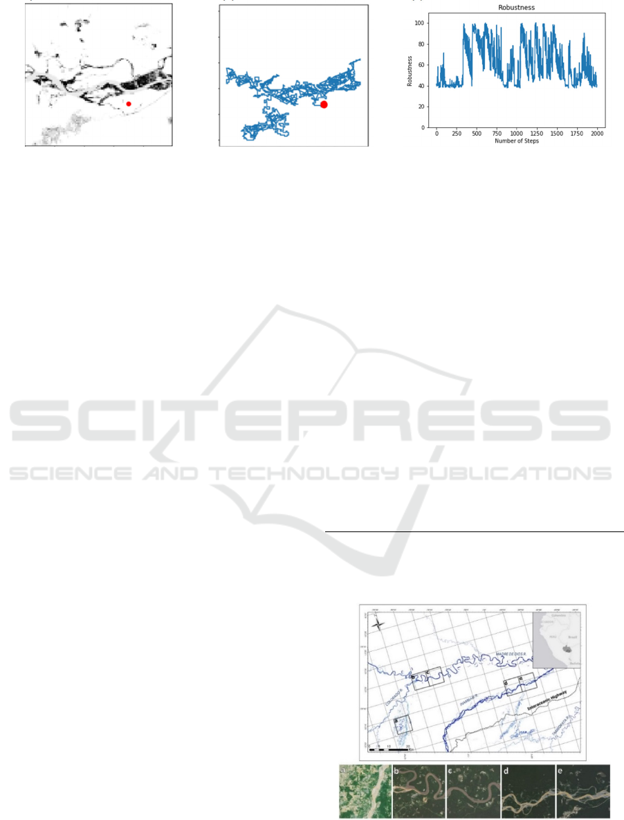
(a)
(b) (c)
Figure 3: (a) Satellite image from Amazon Forest in Peru, (b) Flight trajectory generated by RDE, and (c) robustness value of
the exploration decision at each time step.
would lead the UAV to navigate more AoI while
maintaining its battery constraint. The algorithm
starts by picking a random position to begin the flight.
The algorithm would move the UAV at each time step
to a position with a robustness larger than generated
via the MCMC algorithm (Algorithm1). However,
MCMC is a stochastic algorithm by nature and it
could take many iterations to converge from the
current position to the target position with an
acceptable robustness. Moreover, MCMC runs the
risk of getting stuck in local maxima; areas where the
robustness is higher for the current position than for
its close neighbors, but lower than for locations that
are further away. This could potentially happen when
the UAV explores a large area with little to zero
significant interest. This is remedied by setting a
threshold α to stop the MCMC from generating the
same results and enforce the algorithm to use one of
the cached points, which in this case, represent further
away locations with more robustness values. After
making a decision about the next target, we use RA*,
a path planner algorithm that has been developed
using MTL robustness and A* (Esdaile and Chalker,
2018) to find the path from the current to the next
positions that would give the UAV exposure to more
AoI if there is any around the path.
Back to our ASGM problem, Fig.3(a) shows a
simulated map of the likelihood of finding ASGM for
an area in Amazon forest in Peru. The darker the color
the higher the likelihood is for the area to have
ASGM. Such likelihood values would be provided by
the object detection system onboard the UAV for
small areas within its range of vision. The red circle
represents the starting point of the flight. Fig. 3(b)
shows the flight trajectory that satisfies our RDE
specification in equation 2 and generated by
Algorithm 2 such that AoI is defined as areas of
ASGM. Fig.3(c) plots the robustness of the
exploration decision at each time step. Clearly, the
selected positions for the UAV’s trajectory in the
given map are concentrated in the more promising
regions with higher robustness values above
.
However, the resulting trajectory directly depends on
the starting point and the number of steps which
simulates the battery life of the UAV. More details
about this experiment are shown in next section.
Algorithm 2: RDE Algorithm.
Input: (2): Mission specification, f()=
Robustness
Function
: Robustness threshold,
: neighboring function.
begin
Randomly pick a starting point
While (
)
count=0
While
==
&& count
MCMC(
)
count++
end
if count> && cachedPoints!=
= getCachedPoint();
else
= home;
RA*(
)
End
5 EXPERIMENT
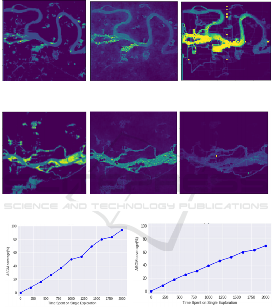
Figure 4: Satellite images for (a) Delta, (b) Colorado, (c)
Madre de Dios, (d) Inambari, (e) La Pampa.
Robustness-driven Exploration with Probabilistic Metric Temporal Logic
63
(a)
(b)
(c)
Figure 5: (a) Distributed ASGM in Colorado region(Figure 4.b), (b) Distribution of most frequent explored locations using
RDE, and (c) Distribution of most frequent explored locations using AEP.
(a)
(b) (c)
Figure 6: (a) Distributed ASGM in La Pampa (Figure 4.e), (b) Distribution of most frequent explored locations using RDE,
and (c) Distribution of most frequent explored locations using AEP.
(a)
(b)
Figure 7: (a) ASGM coverage with RDE (b) ASGM coverage with AE.
The main motivation for this paper is to increase the
UAV’s exploration percentage of ASGM in the
Amazon forest in Peru with limited resources (i.e.
battery and onboard storage). As part of this research,
we have developed an object recognition module
using YOLO (Rubinstein, 1981). Our object
recognition has been trained to detect different
components that are usually found around ASGM
areas such as dredges, floats, sluices, shacks/rooftops,
sand, water, and plantations. The results from the
object recognition have been simulated in this paper
to test the proposed RDE approach.
To help guide the UAV flights to areas with real
information, we implemented our RDE approach over
ICAART 2021 - 13th International Conference on Agents and Artificial Intelligence
64

actual five 8x8 km
2
regions in Peru (.a.Delta,
b.Colorado, c.Madre de Dios, d.Inambari, e. La
Pampa) (Fig.4). We simulate motion of the UAV (as
well as the onboard object detection system) and keep
its altitude fixed by setting the field of view to 200x200
m
2
. We test our RDE approach against the AEP
approach developed in (Selin et al., 2019). However,
due to the space limitation, we only showed the heat
maps for two regions b and e (Colorado, La Pampa).
Fig.5 (a) shows the likelihood of ASGM areas in
the regions b and e shown in (Fig. 4), the color scale
is between yellow and green such that dark yellow
areas have higher probability of having ASGM. Fig.
5 (b) shows the most frequent explored positions in
region b using the proposed RDE approach. We
collected those points by running RDE on 100 trials
with 2000 time steps per each trail starting from
random positions in each run. The green and yellow
colors represent the most visited areas such that areas
in yellow are visited more than areas with green color.
We then explored the same region b using the AEP
(Fig. 4 (c)). The testing results for region e are
illustrated in Fig. 5. For both regions, our approach
was clearly able to navigate the majority of ASGM
areas in comparison to AEP while spending less time
inside vegetation areas. However, AEP was faster in
making decisions than RDE by average of 29% when
exploring the areas shown in Fig.4. AEP uses a
greedy algorithm which guaranteed faster execution
but not necessarily good coverage for ASGM while
RDE needs to compute the robustness of P-MTL
constraints before each exploration decision and use
the MCMC sampler to select the next target with
higher robustness.
Fig.7 illustrates the average coverage of ASGM in
all regions shown in Fig.4 using our RDE and AEP
with different numbers of time steps respectively. The
time steps here represent the battery life for the UAV.
The percentage of coverage grows linearly with the
allotted time for both approaches, but the RDE covers
more ASGM areas by approximately 38% over AEP.
6 CONCLUSIONS
In this paper, we presented a new exploration
approach RDE that incorporates the online discovered
knowledge into the exploration decisions for UAVs.
RDE uses the robustness of P-MTL specifications to
guide the stochastic process of MCMC to make the
exploration decisions in completely unknown
environment. We have tested our approach on four
simulated areas in Amazon forest in Peru to look for
mining areas (e.g. ASGM). In comparison to a greedy
approach called AEP (Selin et al., 2019), our
approach leads the UAV into more areas classified as
ASGM than AEP without getting stuck or spending
long time in vegetation areas. In future work, we
intend to test our approach on real UAVs in Amazon
forest. In order to do that, we have to incorporate the
dynamics of the UAV and the control information
(i.e. speed, altitude) into the P-MTL specifications of
the problem.
REFERENCES
A. Bircher, M. Kamel, K. Alexis, H. Oleynikova, and R.
Siegwart (2016). Receding horizon "Next-Best-View"
planner for 3D exploration. In Proceedings of
International Conference on Robotics and Automation
ICRA, 2016.
A. Dokhanchi, B. Hoxha, and G. Fainekos (2014), On-Line
monitoring for temporal logic robustness.In
Proceedings of International Conference on Runtime
Verification, 2014.
A.I.M Ayala, S.B. Andersson, and C. Belta (2013).
Temporal logic motion planning in unknown
environments. In IEEE/RSJ International Conference
on Intelligent Robots and Systems, 2013.
B. Adler, J. Xiao, and J. Zhang (2014), Autonomous
exploration of urban environments using unmanned
aerial vehicles. Journal of Field Robotics, 2014.
B. Yamauchi (1997). A frontier-based approach for
autonomous exploration. In Proceedings of IEEE
International Symposium on Computational
Intelligence in Robotics and Automation CIRA, 1997.
C. Vasile, J. Tumova, S. Karaman, C. Belta, and D. Rus
(2017). Minimum-violation scLTL motion planning for
mobility-on-demand. In Proceedings of the IEEE
International Conference on Robotics and Automation
(ICRA), 2017
F. S. Barbosa, D. Duberg, P. Jensfelt, and J. Tumova
(2019). Guiding autonomous exploration with signal
temporal logic. In Proceedings of IEEE Robotics and
Automation, 2019.
G. Asner, W. Llactayo, R. Tupayachi, E. Ráez-Luna (2013).
Elevated rates of gold mining in the Amazon revealed
through high-resolution monitoring. In Proceedings of
the National Academy of Sciences of the United States
of America, 2013.
G. Fainekos, and G. Pappas (2006), Robustness of temporal
logic specifications. In Proceedings of the First
combined international conference on Formal
Approaches to Software Testing and Runtime
Verification. 2006.
H. Abbas, G. Fainekos, S. Sankaranarayanan, F. Ivan, and
A. Gupta (2013). Probabilistic Temporal Logic
Falsification of Cyber-Physical Systems. ACM
Transactions on Embedded Computing Systems
(TECS), 2013.
Robustness-driven Exploration with Probabilistic Metric Temporal Logic
65

H. González-Baños, and J. Latombe (2002). Navigation
strategies for exploring indoor environments. The
International Journal of Robotics Research, 2002. p.
829-848.
J. Caballero, M. Messinger, F. Román, C. Ascorra, L.
Fernandez, M. Silman (2018). Deforestation and forest
degradation due to gold mining in the Peruvian
Amazon: A 34-Year perspective. Remote Sensing,
2018.
J. Swenson, C.E Carter, J.C. Domec, C.I, Delgado (2011).
Gold mining in the Peruvian Amazon: global prices,
deforestation, and mercury imports. PLOS ONE, 2011.
L. Esdaile, and J. Chalker (2018), The mercury problem in
artisanal and small-scale gold mining. Chemistry - A
European Journal, 2018.
L. Heng, A. Gotovos, A. Krause, and M. Pollefeys (2015).
Efficient visual exploration and coverage with a micro
aerial vehicle in unknown environments. In
Proceedings of IEEE International Conference on
Robotics and Automation (ICRA), 2015
M. Messinger, G. Asner, and M. Silman (2016). Rapid
assessments of Amazon Forest structure and biomass
using small unmanned aerial systems. Remote Sensing,
2016.
M. Selin, M. Tiger, D. Duberg, F. Heintz, and P. Jensfelt
(2019). Efficient autonomous exploration planning of
large-scale 3-D environments. In Proceedings of IEEE
Robotics and Automation Letters.
M. Tiger, and F. Heintz (2016). Stream reasoning using
temporal logic and predictive probabilistic state
models . In Proceedings of 23rd International
Symposium on Temporal Representation and
Reasoning (TIME), 2016.
Redmon, J., et al. You Only Look Once: Unified, Real-
Time Object Detection. in 2016 IEEE Conference on
Computer Vision and Pattern Recognition (CVPR).
2016.
R. Koymans (1990). Specifying real-time properties with
metric temporal logic. Real-Time Systems.1990. p.
255-299.
Rubinstein, R.Y., Simulation and the Monte Carlo Method.
1981: John Wiley \& Sons, Inc. 304.
S. Alqahtani, I. Riley, S. Taylor, R. Gamble, and R, Mailler
(2018). MTL robustness for path planning with A*. In
Proceedings of the 17th International Conference on
Autonomous Agents and MultiAgent Systems. 2018. p.
247-255
S. Chib, and E. Greenberg (1995). Understanding the
Metropolis-Hastings algorithm. American Statistician,
1995.
S. Karaman, and E. Frazzoli (2009). Sampling-based
motion planning with deterministic μ-calculus
specifications. In Proceedings of the IEEE Conference
on Decision and Control (CDC), 2009.
S. Karaman, and E. Frazzoli (2011), Sampling-based
algorithms for optimal motion planning. The
International Journal of Robotics Research, 2011. p.
846-894.
ICAART 2021 - 13th International Conference on Agents and Artificial Intelligence
66
