Improving the Grid-based Clustering by Identifying Cluster Center
Nodes and Boundary Nodes Adaptively
Yaru Li, Yue Xi and Yonggang Lu
School of Information Science and Engineering, Lanzhou University, Lanzhou, 730000, China
Keywords: Grid-based Clustering, Density Estimation, Boundary Nodes, Clustering Analysis.
Abstract: Clustering analysis is a data analysis technology, which divides data objects into different clusters according
to the similarity between them. The density-based clustering methods can identify clusters with arbitrary
shapes, but its time complexity can be very high with the increasing of the number and the dimension of the
data points. The grid-based clustering methods are usually used to deal with the problem. However, the
performance of these grid-based methods is often affected by the identification of the cluster center and
boundary based on global thresholds. Therefore, in this paper, an adaptive grid-based clustering method is
proposed, in which the definition of cluster center nodes and boundary nodes is based on relative density
values between data points, without using a global threshold. First, the new definitions of the cluster center
nodes and boundary nodes are given, and then the clustering results are obtained by an initial clustering
process and a merging process of the ordered grid nodes according to the density values. Experiments on
several synthetic and real-world datasets show the superiority of the proposed method.
1 INTRODUCTION
Clustering analysis is well known as an unsupervised
machine learning method, which is a process of
dividing the given set of data objects into different
subsets according to some criteria. Each subset is a
cluster, so that data objects in the same subset have a
higher similarity, while data objects belonging to
different subsets have a lower similarity (Jain et al.,
1999). Clustering analysis has been widely used in
many fields, including pattern recognition, image
analysis, Web search, biology, etc. (Liaoet al., 2012).
Clustering analysis is a very challenging research
field. With the development of clustering analysis, a
large number of clustering methods have been
proposed, most of them can be divided into two
groups: partitioning based clustering and hierarchical
based clustering (Jain, 2010). The partition-based
clustering methods include centroid-based clustering
methods, density-based clustering methods, grid-
based clustering methods and model-based clustering
methods, etc.
For centroid-based clustering methods, they can
obtain clusters according to the relationship between
the centroid of clusters and data objects. A majority
of centroid-based clustering methods are easy to
understand and implement, but they can only
recognize spherical clusters, due to the fact that the
distance between data objects is utilized to divide
datasets, such as K-means (MacQueen, 1967), K-
medoids (Kaufman and Rousseeuw, 2009), etc.
Moreover, in the centroid-based clustering methods,
the value of K needs to be preset, and the selection of
initial clustering centers have a significant influence
on the final clustering results.
Unlike centroid-based clustering, the density-
based clustering methods can recognize clusters with
arbitrary shapes instead of identifying only spherical
clusters, they can also automatically obtain the
appropriate number of clusters without presetting the
number of clusters, and they are not sensitive to noise
and outliers. The basic idea of the density-based
methods is that high-density areas are separated by
low-density areas, and data objects in the same
density area belong to the same cluster. The most
popular density-based clustering methods are
DBSCAN (Ester, et al., 1996), DENCLUE (Campello
et al., 2015), DPC (Rodriguez and Laio, 2014), etc.
At present, most density-based clustering methods
may not consider datasets with large differences in
density distribution when calculating the density,
which may lead the data points to be clustered
incorrectly. Therefore, many clustering methods are
182
Li, Y., Xi, Y. and Lu, Y.
Improving the Grid-based Clustering by Identifying Cluster Center Nodes and Boundary Nodes Adaptively.
DOI: 10.5220/0010191101820189
In Proceedings of the 10th International Conference on Pattern Recognition Applications and Methods (ICPRAM 2021), pages 182-189
ISBN: 978-989-758-486-2
Copyright
c
 2021 by SCITEPRESS – Science and Technology Publications, Lda. All rights reserved

proposed, which can solve the problem to a certain
extent, such as DDNFC (Liu et al., 2020), DPC-
SFSKNN (Diao et al., 2020), etc. Another drawback
of density-based clustering methods is that with the
increase of the dimensions or the number of data
objects, density-based clustering methods will be
limited by time complexity and space complexity.
The grid-based clustering methods can reduce the
time complexity of the clustering process because a
mapping relationship is established between data
objects and grids, all clustering operations only need
to be performed on the grid. Grid-based clustering
methods firstly embed data objects into disjoint grids,
then the grids are clustered by specific methods,
finally, the data objects are labeled according to the
relationship between grids and data objects. The
common grid-based clustering methods are STING
(Wang et al., 1997), GRIDCLUS (Schikuta, 1996),
etc. However, the accuracy of clustering results will
vary due to different grid partitions.
Therefore, the clustering methods based on both
grid and density have been proposed to get more
accurate clustering results in a shorter time. Rakesh et
al. proposed the CLIQUE method (Agrawal et al.,
1998), in which the result of clustering is obtained by
finding the maximum dense units in the subspace. Wu
et al. put forward a new method for calculating the
density of grid nodes, which improves the density
calculation method of the grid in the CLIQUE method
(Wu and Wilamowski, 2016). Xu et al. put forward a
density peaks clustering method based on grid
(DPCG) (Xu et al., 2018), which employs the grid
division in the CLIQUE method for reducing the time
complexity of the DPC method when computing the
local density. However, a common shortcoming of
these grid-based clustering methods is that the
definition of the cluster center and boundary are both
based on some global thresholds, and the whole
clustering process will be affected by the selection of
cluster center and the determination of boundary.
Therefore, the setting of the global thresholds will
have a significant impact on the final clustering result
for the methods.
In order to solve the above problems, this paper
proposes an adaptive clustering method based on both
grid nodes and density estimation. In the method, a
new definition of cluster center nodes and boundary
nodes based on the relative density value is given
which doesn’t depend on a global threshold, and then
a new clustering process is proposed, which consists
of an initial clustering process and a merging process.
Experiments on eight UCI datasets and two synthetic
datasets show the effectiveness of the proposed
method.
The rest of this paper is organized as follows: an
adaptive clustering method based on both grid nodes
and density estimation is proposed in Section 2. The
experimental results will be shown in Section 3. The
conclusion is given in Section 4.
2 THE PROPOSED METHOD
In this section, an adaptive clustering method based
on both grid nodes and density estimation (CBGD) is
proposed, which includes two stages: preprocessing
and clustering. Compared with the traditional
clustering methods based on the grid, the density
calculation of grid nodes is used in CBGD, which can
simplify the establishment of the mapping
relationship between grids and data objects and can
reduce the time complexity of the algorithm.
Furthermore, there is no necessity to preset global
thresholds for identifying cluster center nodes and
boundary nodes in the CBGD method, which avoids
the disadvantage brought by the global thresholds on
the clustering results. A detailed description of each
stage is shown below.
2.1 The First Stage: Preprocessing
In the first stage, it includes three steps to prepare for
clustering: partitioning grids, scaling data objects into
grids, and calculating the density of grid nodes. The
specific description of each step is introduced in the
following part.
2.1.1 Partitioning Grids, Scaling Data
Objects into Grids
At first, the feature value of the data objects in each
dimension is scaled to between 1 and grid_num,
where grid_num is the parameter for partitioning
grids (Wu and Wilamowski, 2016). The grid is
obtained by rounding the scaled value of the data
objects in each dimension. In the two-dimensional
space, the grid is a square with length and width of
one, and the grid nodes are the four vertices of the
square. In the three-dimensional space, the grid is a
cube with length, width, and height equal to one, and
the grid nodes are the eight vertices of the cube.
Obviously, the dimension of grids is equal to the
number of features of the dataset, and the distance
between two adjacent grid nodes is equal to one,
which can provide a great convenience for the
subsequent clustering process.
Improving the Grid-based Clustering by Identifying Cluster Center Nodes and Boundary Nodes Adaptively
183

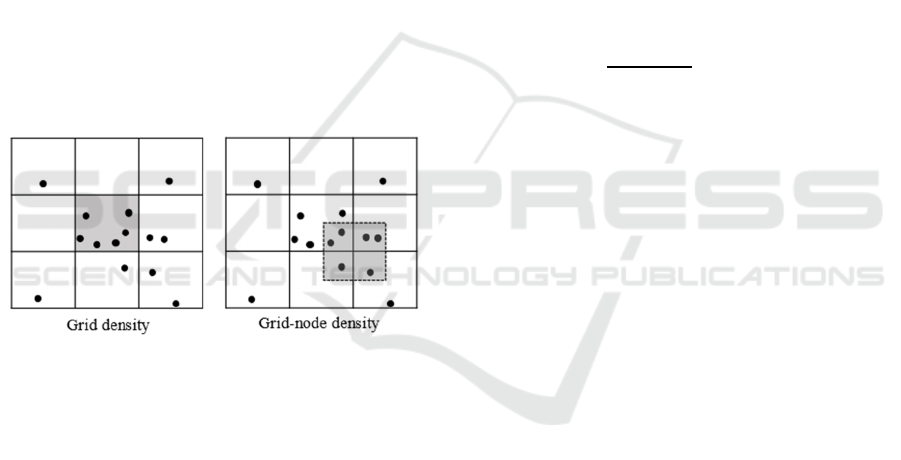
2.1.2 Calculating the Density of Grid Nodes
In grid-based clustering methods, there are two
common methods for calculating local density. The
first is to calculate the local density of the grid, and
the second is to calculate the local density of grid
nodes. The difference between these two density
calculation methods is shown in Figure 1. The left
side of the figure is the density calculation method of
the grid, the gray area represents a grid, and its density
is defined as the number of data objects falling into
the grid. The right of the figure is the density
calculation method of the grid nodes, its density is the
same as the density calculation method of the grid,
which is also defined as the number of data objects
falling into the gray area. In most traditional grid-
based clustering methods, the first one is selected to
calculate the local density, therefore, in order to
calculate the density of grids, the relationship
between data objects and grids must be estimated to
determine which grid the data object should fall into.
In this paper, in order to simplify the calculation of
grid density, the density of grid nodes is applied in the
proposed method.
Figure 1: Density calculation methods of the grid (left) and
grid-node (right).
2.2 The Second Stage: Clustering
In this section, first, a new definition of the cluster
center nodes and boundary nodes based on the
relative density value is given, and then a new
clustering process of CBGD is shown in detail, which
consists of an initial clustering process and a merging
process based on cluster-interconnectivity.
2.2.1 Definitions
Definition 1 (Neighboring Node). A node X is
defined as a neighboring node of node Y if node X is
adjacent to node Y, that is, the distance between X and
Y is one.
Definition 2 (Successor Node). A node X is defined
as a successor node of node Y if X is a unlabeled
neighboring node of Y and the density value of X is
smaller than the density value of Y.
Definition 3 (Boundary Node). A node that is a
successor node of another node, but has no successor
nodes.
Definition 4 (Cluster Center Node). The node having
the largest density value in a cluster is defined as the
cluster center node.
Definition 5 (Cluster-boundary Node). For a
boundary node X in a cluster C
i
, and a cluster C
j
C
i
,
if dist (X, C
j
) < dist (C
i
, C
j
), the node X is defined as
a cluster-boundary node between C
i
and C
j
.
Where dist (X, C
j
) is the distance between node X
and the cluster center node of cluster C
j
, dist (C
i
, C
j
)
is the distance between the cluster center nodes of the
cluster C
i
and C
j
.
Definition 6 (Cluster-interconnectivity). According
to the cluster-boundary node, we define the cluster-
interconnectivity between any two clusters C
i
and C
j
as:


,

 = 
1
max
|

|
,
|

|
,  

,

 
0 ,
(1)
where | X | is the number of cluster-boundary nodes
between cluster C
i
and C
j
in cluster C
i
, | Y | is the
number of cluster-boundary nodes between cluster C
i
and C
j
in cluster C
j
, dist(C
i
, C
j
) is the distance between
the cluster center nodes of the cluster C
i
and C
j
, δ is
the maximum distance at which two clusters are
likely to merge. The cluster-interconnectivity
represents the possibility of the different subclusters
belong to the same cluster. The higher the cluster-
interconnectivity between two subclusters, the greater
the probability that they belong to the same cluster.
2.2.2 Initial Clustering Process
Before the initial clustering, firstly, the grid nodes
need to be sorted by the density values obtained in the
first stage from the highest to the lowest, and then the
sorted grid nodes are clustered according to the order
in turn. The idea of initial clustering is that the
adjacent grid nodes belong to the same cluster. If a
grid node has already been clustered, then the grid
nodes that are adjacent to it and are not clustered
should also be added to the cluster that it belongs to.
If a grid node has not been clustered, a new cluster
should be created for it and its unlabeled neighboring
grid nodes. The specific description of the initial
clustering process is given in Algorithm 1.
ICPRAM 2021 - 10th International Conference on Pattern Recognition Applications and Methods
184

2.2.3 Merging Process
After the initial clustering process, for sparsely
distributed clusters, data objects that originally
belong to the same cluster may be divided into
multiple clusters, so it is necessary to merge the
clusters obtained in the initial clustering process to
get more accurate results. Before the merging
process, the distance between different clusters needs
to be calculated in advance. In this paper, the distance
between clusters is defined as the distance between
cluster center nodes, and there are two conditions for
the merging process: a closer distance and a higher
cluster-interconnectivity between the clusters.
Therefore, in order to merge clusters, these two
conditions must be satisfied. In our experiments, the
Euclidean distance is used as the distance measure for
all the datasets.
Algorithm 1: Initial Clustering Process.
INPUT
N
odes - a set containing n grid nodes.
D
ensity - density of grid nodes.
OUTPUT
L
abels - initial clustering results of gri
d
nodes.
1. SortedIndex ← the sorted index of the grid nodes
according to density value from the highest to the
lowest.
2. Mark all grid nodes as unvisited.
3. FOR i ← 1 to n DO
4. Let N be the set of unlabeled neighboring nodes of
sortedIndex[i].
5. IF N is not empty THEN
6. Mark all grid nodes in N as visited.
7. IF sortedIndex[i] is visited
8. Label[N] = Label[sortedIndex[i]].
9. ELSE
10. Mark sortedIndex[i] as visited.
11. Create a new cluster C
i
and assign the new
cluster label to both sortedIndex[i] and the grid
nodes in N.
12. ELSE
13. Mark sortedIndex[i] as boundary node.
14. IF sortedIndex[i] is unvisited
15. Mark sortedIndex[i] as visited.
16. Create a new cluster C
i
and assign the new
cluster label to the sortedIndex[i].
17. END FOR
In the process of the merging, the clusters with a
smaller distance are selected at first, and then the
cluster-interconnectivity between these clusters is
calculated according to the formula (1). If the cluster-
interconnectivity between these clusters is greater
than the given threshold, they will be merged. The
specific description of the merging process is given in
Algorithm 2.
After obtaining the final clustering result of grid
nodes, the clustering result of the original dataset can
be obtained by assigning the cluster label of grid
nodes to data objects according to the corresponding
relationship between grid nodes and data objects.
Algorithm 2: Merging Process.
INPUT
L
abels - initial cluster label of grid nodes.
Clusters - a set containing m clusters.
δ- the maximum distance at which two
clusters are likely to merge.
α - cluster-interconnectivity threshold.
OUTPUT
F
inal_Labels - the final clustering result o
f
grid nodes.
1. Final_Labels ← Labels.
2. FOR i ←1 to m DO
3. Let L be the set of clusters whose distance from
the Clusters[i] is smaller than δ.
4. FOR j ←1 to |L| DO
5. X ← the cluster-boundary nodes between
Clusters[i] and L[j] in Clusters[i].
6. Y ← the cluster-boundary nodes between
Clusters[i] and L[j] in L[j].
7. CI (i, j) ← the CI (Clusters[i], L[j]) computed
using (1).
8. IF CI (i, j) > 1/α
9. Final_Labels[L[j]] ← Labels[Clusters[i]].
10. END FOR
11. END FOR
3 EXPERIMENTAL RESULTS
In order to demonstrate the effectiveness of the
proposed method, the clustering results of the
proposed method are compared with those of the
three other methods: DBSCAN (Ester et al., 1996),
DPC (Rodriguez and Laio, 2014), and DPCG (Xu et
al., 2018).
3.1 Datasets
In the experiments, eight UCI real-world datasets and
two synthetic datasets are used to evaluate the
effectiveness of the proposed method. These datasets
have different sizes and dimensions. A detailed
description of these datasets is given in Table 1.
3.2 Evaluation Criterion
In this paper, two common evaluation criteria are
used to evaluate the clustering results obtained by the
proposed method: Adjusted Rand Index (ARI)
(Hubert and Arabie, 1985) and Fowlkes-Mallows
Improving the Grid-based Clustering by Identifying Cluster Center Nodes and Boundary Nodes Adaptively
185

Index (FM-Index) (Fowlkes and Mallows, 1983). The
value ranges of FM_Index is [0,1], and the value
ranges of ARI is [-1,1], for both of them, the larger
the value, the better the clustering results. The
calculation formulas of these two evaluation criteria
are defined as follows:
_






(2)


max




(3)
where TP is the number of pairs of data points that are
in the same cluster in both ground truth and the
clustering result, TN is the number of pairs of data
points that are in different clusters in both ground
truth and the clustering result, FN is the number of
pairs of data points that are in different clusters in the
clustering result but in the same cluster in the ground
truth, FP is the number of pairs of data points that are
in the same cluster in the clustering result but in
different clusters in the ground truth, and 
 


⁄
, 


is the number of point pairs that
can be formed in the dataset, E[RI]is the expected
value of the RI.
Table 1: A detailed description of the datasets in the
experiments.
Datasets N
a
D
b
M
c
Source
Pathbased 300 2 3 Synthetic dataset
Jain 373 2 2 Synthetic dataset
Iris 150 4 3 UCI datasets
d
Seeds 210 7 3 UCI datasets
Glass 214 9 7 UCI datasets
Breast 699 9 2 UCI datasets
Wine 178 13 3 UCI datasets
Abalone 4177 8 3 UCI datasets
Thyroid 215 5 3 UCI datasets
Modeling 258 5 4 UCI datasets
a
The number of the data objects.
b
The dimension of the datasets.
c
The actual number of clusters in the datasets.
d
http://archive.ics.uci.edu/ml/datasets/.
3.3 Parameters Selection
In the experiments, there are three important
parameters that need to be determined: grid_num, the
number of grids in each dimension; δ, the maximum
distance at which two clusters are likely to merge; and
α, the threshold of cluster-interconnectivity, which is
the percentage of the number of cluster-boundary
nodes to the number of data objects in the datasets.
The formula grid_num=round(
√


+5) is used to
determine the number of grids in each dimension
(Wang, Lu, and Yan, 2018), except two-dimensional,
where d is the number of features and n is the number
of data objects of the dataset.
The maximum distance δ, which is used to
calculate the cluster-interconnectivity between
clusters in formula (1), has a direct impact on the
quality of the experimental results. If the value of δ is
too large, the clusters obtained in the initial clustering
process may be merged into the same cluster during
the merging process, when the value of δ is too small,
it is difficult to merge the subclusters belonging to the
same clusters. If the cluster-interconnectivity
between two clusters greater than α, these two
clusters should be merged; otherwise, they should not
be merged.
Due to difficulties in finding a general method to
determine the value of the parameters
for all datasets,
for a fair comparison, the parameters which produce
the best clustering results in the experiments are
selected for all the four clustering methods. The
parameters selected for each of the methods
corresponding to each dataset are shown in Table 2.
Table 2: The setting of parameters of each method in the
experiments.
Datasets DPC DBSCAN DPCG CBGD
(d
c
)
(Minpts/ε)
(d
c
/a) (δ/α)
Pathbased 1.10 10.0/2.00 4.8/0.01 5.1/1.00
Jain 0.90 3.0/2.35 0.2/0.10 3.2/1.10
Iris 0.07 4.0/0.90 2.9/0.20 2.5/2.00
Seeds 0.70 2.0/0.89 2.0/0.10 2.5/1.40
Glass 1.70 11.0/1.39 0.2/0.50 2.5/1.40
Breast 0.70 11.0/3.90 2.0/0.30 3.4/0.30
Wine 2.00 7.0/0.51 3.4/1.00 3.5/1.60
Abalone 0.30 5.0/1.00 0.1/0.10 5.0/1.20
Thyroid 0.01 2.0/3.70 0.1/0.90 3.2/0.90
Modeling 0.01 2.0/2.50 2.3/0.50 3.5/1.50
3.4 Comparison of Clustering Results
3.4.1 Synthetic Datasets
In this part, the proposed method is compared with
three different clustering methods on two artificial
datasets, which have different shapes, sizes and
distributions. The final clustering results are shown in
Figure 2, Figure 3. From the figure, we can clearly see
the cluster distribution of datasets and the clustering
ICPRAM 2021 - 10th International Conference on Pattern Recognition Applications and Methods
186

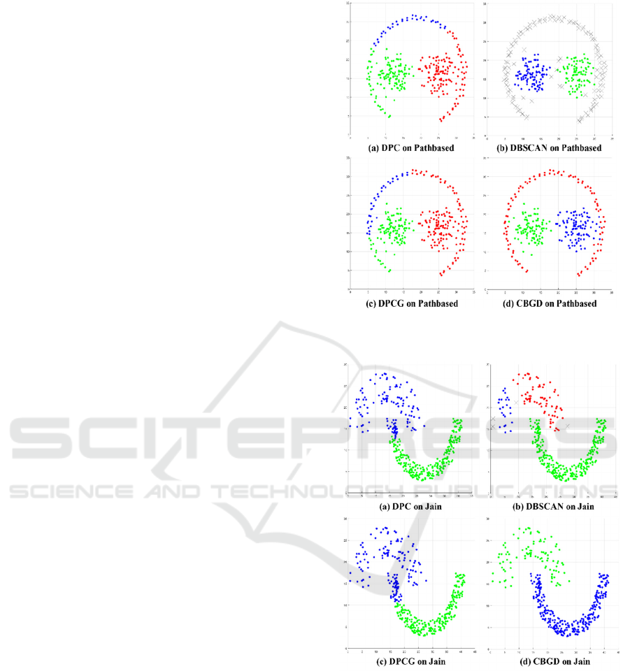
results of each clustering method for different
datasets.
The pathbased (Chang and Yeung, 2008) dataset
is composed of 300 data objects, which are divided
into three clusters, the arc is a cluster, and the other
two clusters are surrounded by the arc. As shown in
Figure 2, we can find that although the DPC method
can identify three clusters, due to its clustering
method: assigning remaining data points to the same
clusters as its nearest neighbor with higher density
after cluster centers are selected, so the data points at
the lower left and lower right of the arc-cluster are
incorrectly assigned to the other two clusters. For the
DBSCAN clustering method, the arc-cluster is
recognized as noise, because the distribution of the
arc-cluster is sparser than the other two clusters. In
the clustering results of the DPCG method is similar
to that of DPC, the data points at the lower left and
lower right of the arc-cluster are also incorrectly
assigned to the other two clusters. Compared with the
other three methods, the CBGD method can correctly
identify three clusters, and only a few data points on
the edge of the cluster are identified incorrectly.
Figure 3 shows the clustering results of four
clustering methods on the Jain (Jain and Law, 2005)
dataset. The Jain dataset contains 373 data points,
which are distributed in the shape of two crescents,
each crescent representing a cluster. Because the
density of the two clusters is quite different, in the
DPC method, the two cluster centers are both selected
in the lower cluster, which makes some points
belonging to the lower cluster wrongly assigned to the
upper cluster. In the clustering results of DBSCAN,
the whole dataset is divided into three clusters. The
lower cluster is completely correct, but the upper
cluster is divided into two different clusters. The
clustering result of the DPCG method is almost the
same as that of DPC method. The CBGD method can
accurately divide the dataset into upper and lower
crescent-clusters.
The FM-Index and Adjusted Rand-Index
produced by four clustering methods on synthetic
datasets are provided in Table 3 and Table 4. Based
on the above clustering results, we can find that the
performance of the CBGD method on artificial
datasets is better than the other three clustering
methods.
Figure 2: The clustering results of the four methods on the
Pathbased dataset.
Figure 3: The clustering results of the four methods on the
Jain dataset.
3.4.2 Real-world Datasets
In this section, eight UCI datasets are used in the
experiment. The FM-index and Adjusted Rand-index
produced by the four clustering methods on these
datasets are shown in Table 5 and Table 6
respectively.
Improving the Grid-based Clustering by Identifying Cluster Center Nodes and Boundary Nodes Adaptively
187

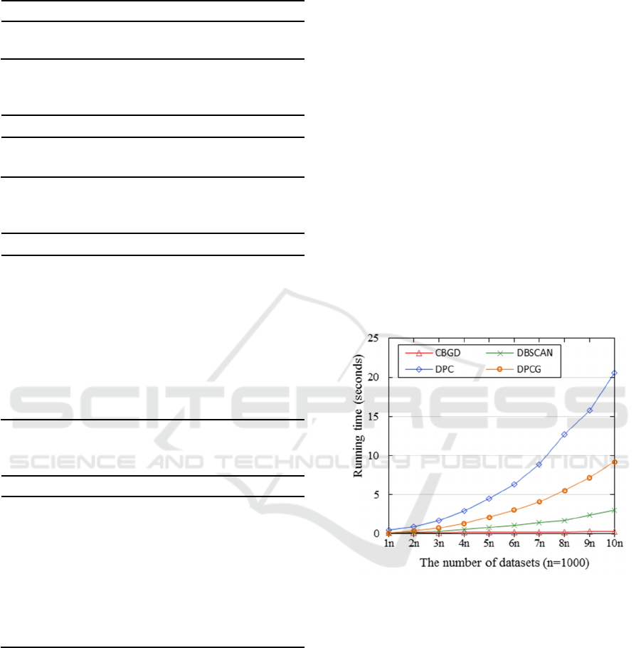
Table 3: The FM-Indices produced by four clustering
methods on synthetic datasets.
Datasets DPC DBSCAN DPCG CBGD
Pathbased 0.6654 0.9205 0.6842
0.9406
Jain 0.8818 0.9765 0.8160
1.0000
Table 4: The Adjusted Rand-Indices produced by four
clustering methods on synthetic datasets.
Datasets DPC DBSCAN DPCG CBGD
Pathbased 0.4678 0.8805 0.4923
0.9111
Jain 0.7146 0.9405 0.5691
1.0000
Table 5: The FM-Indices produced by four clustering
methods on real-world datasets.
Datasets DPC DBSCAN DPCG CBGD
Iris 0.9233 0.7715 0.9345
0.9356
Seeds
0.8444
0.6422 0.7267 0.7783
Glass 0.4408 0.5655 0.5363
0.5760
Breast 0.7192 0.9072 0.7802
0.9188
Wine 0.7834 0.6621
0.8006
0.6586
Abalone 0.5153 0.2250 0.4910
0.5785
Thyroid 0.6638 0.8731 0.7927
0.8754
Modeling 0.6192 0.6981 0.7058
0.7085
Table 6: The Adjusted Rand-Indices produced by four
clustering methods on real-world datasets.
Datasets DPC DBSCAN DPCG CBGD
Iris 0.8857 0.5681 0.8857
0.9039
Seeds
0.7669
0.3975 0.5552 0.6664
Glass 0.1499 0.2579 0.2106
0.2948
Breast 0.4089 0.7973 0.4158
0.8241
Wine 0.6723 0.4468
0.6958
0.5137
Abalone 0.0848 0.0386
0.1349
0.0053
Thyroid 0.4153 0.6949 0.5510
0.6958
Modeling 0.0023
0.0107
-0.0008 -0.001
It can be seen from Table 5 that the FM-Index of
the CBGD method is greater than that of other
methods on all datasets except seeds and wine
datasets. For the seeds dataset, the FM-Index of the
CBGD method is the second-best one. From Table 6
we can see that the Adjusted Rand-Index of the
CBGD method is greater than that of other methods
on four datasets, for the seeds dataset, the Adjusted
Rand-Index of the CBGD method is the second-best,
however, on the other three datasets, the Adjusted
Rand-Index of the CBGD method is slightly poor
than other methods.
In addition, for showing the efficiency of the
CBGD method, the datasets with the number of data
objects ranging from 1000 to 10000 are used to test
the time complexity of the four clustering methods,
the average running time of 10 experiments is
selected as the final running time for each method.
The experimental results are shown in Figure 4.
From Figure 4, it can be seen that the time
complexity of the DPC method increases roughly
exponentially which is significantly higher than that
of other clustering methods. When the number of data
objects is between 1000 and 2000, the difference of
running time between DBSCAN, DPCG, and CBGD
is very small. With the increase in the number of data
points, the running time of the DPCG method is
higher than that of the other two methods. Especially,
when the number of data points is greater than 5000,
the difference of the running time between the grid-
based clustering method DPCG and the proposed
method CBGD gradually increase.
Figure 4: The comparison of the time complexity of the four
methods.
Based on the above experimental results, we can
find that regardless of the FM-Index and Adjusted
Rand-Index of the clustering results or the running
time of the methods, the CBGD method is superior to
the other three clustering methods.
4 CONCLUSIONS
In this paper, an adaptive clustering method based on
both grid nodes and density estimation (CBGD) is
proposed. In this method, a new definition of the
cluster center nodes and boundary nodes is given that
ICPRAM 2021 - 10th International Conference on Pattern Recognition Applications and Methods
188

doesn’t depend on a global threshold, which avoids
the disadvantage brought by other grid-based
methods. Experimental results show that the proposed
CBGD method is superior to other methods in
clustering performance and time complexity. It can be
seen that the identification of the cluster center and
boundary are important for the clustering process. An
adaptive method for identifying cluster center and
boundary nodes is better than the methods based on
global thresholds. In future work, we will study how
to improve the proposed method by designing a better
grid partition method.
ACKNOWLEDGEMENTS
This work is supported by the Fundamental Research
Funds for the Central Universities (Grants No.
lzuxxxy-2019-tm10).
REFERENCES
Jain, A. K., Murty, M. N., & Flynn, P. J., 1999. Data
clustering: a review. ACM computing surveys, 31(3),
264-323.
Liao, S. H., Chu, P. H., & Hsiao, P. Y., 2012. Data mining
techniques and applications–A decade review from
2000 to 2011. Expert systems with applications, 39(12),
11303-11311.
Jain, A. K., 2010. Data clustering: 50 years beyond K-
means. Pattern recognition letters, 31(8), 651-666.
MacQueen, J., 1967. Some methods for classification and
analysis of multivariate observations. In Proceedings of
the fifth Berkeley symposium on mathematical statistics
and probability (Vol. 1, No. 14, pp. 281-297).
Kaufman, L., & Rousseeuw, P. J., 2009. Finding groups in
data: an introduction to cluster analysis (Vol. 344).
John Wiley & Sons.
Ester, M., Kriegel, H. P., Sander, J., & Xu, X., 1996.
Density-based spatial clustering of applications with
noise. In Int. Conf. Knowledge Discovery and Data
Mining, Vol. 240, p. 6.
Campello, R. J., Moulavi, D., Zimek, A., & Sander, J.,
2015. Hierarchical density estimates for data clustering,
visualization, and outlier detection. ACM Transactions
on Knowledge Discovery from Data, 10(1), 1-51.
Rodriguez, A., & Laio, A., 2014. Clustering by fast search
and find of density peaks. Science, 344(6191), 1492-
1496.
Liu, Y., Liu, D., Yu, F., & Ma, Z., 2020. A Double-Density
Clustering Method Based on “Nearest to First in”
Strategy. Symmetry, 12(5), 747.
Diao, Q., Dai, Y., An, Q., Li, W., Feng, X., & Pan, F., 2020.
Clustering by Detecting Density Peaks and Assigning
Points by Similarity-First Search Based on Weighted
K-Nearest Neighbors Graph. Complexity, 2020,
1731075:1-1731075:17.
Wang, W., Yang, J., & Muntz, R., 1997. STING: A
statistical information grid approach to spatial data
mining. In VLDB (Vol. 97, pp. 186-195).
Schikuta, E., 1996. Grid-clustering: an efficient hierarchical
clustering method for very large data sets. Proceedings
of 13th International Conference on Pattern
Recognition, 2, 101-105 vol.2.
Agrawal, R., Gehrke, J. E., Gunopulos, D., & Raghavan, P.,
1998. Automatic subspace clustering of high
dimensional data for data mining applications. Data
Mining & Knowledge Discovery, 27(2), 94-105.
Wu, B., & Wilamowski, B. M., 2016. A fast density and
grid based clustering method for data with arbitrary
shapes and noise. IEEE Transactions on Industrial
Informatics, 13(4), 1620-1628.
Xu, X., Ding, S., Du, M., & Xue, Y., 2018. DPCG: an
efficient density peaks clustering algorithm based on
grid. International Journal of Machine Learning and
Cybernetics, 9(5), 743-754.
Hubert, L., & Arabie, P., 1985. Comparing partitions.
Journal of classification, 2(1), 193-218.
Fowlkes, E. B., & Mallows, C. L., 1983. A method for
comparing two hierarchical clusterings. Journal of the
American statistical association, 78(383), 553-569.
Wang, L., Lu, Y., & Yan, H., 2018. A Fast and Robust Grid-
Based Clustering Method for Dataset with Arbitrary
Shapes. In FSDM (pp. 636-645).
Chang, H., & Yeung, D. Y., 2008. Robust path-based
spectral clustering. Pattern Recognition, 41(1), 191-
203.
Jain, A. K., & Law, M. H., 2005. Data clustering: A user’s
dilemma. In International conference on pattern
recognition and machine intelligence (pp. 1-10).
Springer, Berlin, Heidelberg.
Improving the Grid-based Clustering by Identifying Cluster Center Nodes and Boundary Nodes Adaptively
189