Active Output Selection Strategies for Multiple Learning
Regression Models
Adrian Prochaska
1 a
, Julien Pillas
1
and Bernard Bäker
2
1
Mercedes-Benz AG, 71059 Sindelfingen, Germany
2
TU Dresden, Chair of Vehicle Mechatronics, 01062 Dresden, Germany
Keywords:
Gaussian Processes, Active Learning, Regression, Active Output Selection, Drivability Calibration.
Abstract:
Active learning shows promise to decrease test bench time for model-based drivability calibration. This paper
presents a new strategy for active output selection, which suits the needs of calibration tasks. The strategy
is actively learning multiple outputs in the same input space. It chooses the output model with the highest
cross-validation error as leading. The presented method is applied to three different toy examples with noise in a
real world range and to a benchmark dataset. The results are analyzed and compared to other existing strategies.
In a best case scenario, the presented strategy is able to decrease the number of points by up to 30 % compared
to a sequential space-filling design while outperforming other existing active learning strategies. The results are
promising but also show that the algorithm has to be improved to increase robustness for noisy environments.
Further reasearch will focus on improving the algorithm and applying it to a real-world example.
1 INTRODUCTION
Active learning methods – sometimes called online
design of experiments or optimal experimental design
– increase the capabilities of algorithms taking part in
test design and execution (Cohn, 1996). They reduce
the required number of measurements significantly,
while guaranteeing adequate model qualities (Klein
et al., 2013). However, most methods aim at opti-
mally identifying only one model. In most real-world
applications, there are not one but multiple outputs.
That leaves the test engineer with a question: Should
all models be learned sequentially or simultaneously?
And if they learn simultaneously, how to decide which
model is the leading one? Drivability calibration appli-
cations can be further distinguished from other active
learning tasks because
• the goal is to identify all measured outputs equally
well and
• pulling one query reveals the values of all outputs
of interest.
(Dursun et al., 2015) showed a comparison of a sequen-
tial and a round-robin learning strategy for a drivability
calibration task. To the authors knowledge, no other
publication analyses more sophisticated strategies for
a
https://orcid.org/0000-0003-2707-1266
multiple learning regression models, which follow the
conditions described above. This paper proposes a
new concept of learning strategy, which decides on
the leading output by evaluating a cross validation er-
ror. This new strategy is compared to other existing
strategies. Multiple toy examples are used to create a
noisy but reproducible test environment with different
complexities. At last, the strategy is also applied to a
benchmark dataset.
The paper is structured in six sections. Section 2 of
this paper introduces previous works in context of ac-
tive learning in general and in particular for regression
tasks. Section 3 focuses on describing the specialties
of active learning in the calibration context. A new ac-
tive learning task called active output selection (AOS)
is introduced there. Section 4 describes the analyzed
approaches. Furthermore, a new approach for AOS is
presented. The approaches are evaluated using a toy
example and a benchmark dataset. Experimental de-
tails and a discussion of results are shown in section 5.
At the end, section 6 concludes the results and presents
fields of possible future works.
150
Prochaska, A., Pillas, J. and Bäker, B.
Active Output Selection Strategies for Multiple Learning Regression Models.
DOI: 10.5220/0010181501500157
In Proceedings of the 10th International Conference on Pattern Recognition Applications and Methods (ICPRAM 2021), pages 150-157
ISBN: 978-989-758-486-2
Copyright
c
 2021 by SCITEPRESS – Science and Technology Publications, Lda. All rights reserved

2 PREVIOUS WORK
The field of active learning is a growing branch of the
very present machine learning domain. It is also re-
ferred to as optimal experimental design (Cohn, 1996).
(Settles, 2009) shows a broad overview of the cur-
rent state of the art in this discipline and gives an
outlook to multiple possible future work fields. Recent
methodological advances in the scientific community
mainly focused on classification problems. The main
application domains are speech recognition and text
information extraction (Settles, 2009).
While regression tasks in the context of active
learning have not been as popular, the methodolog-
ical development is relevant as well. (Sugiyama and
Rubens, 2008) propose an approach which actively
learns multiple models for the same task and picks
the best one to query new points. (Cai et al., 2013)
introduced an approach which uses expected model
change maximization (EMCM) to improve the active
learning progress for gradient boosted decision trees,
which was later extended to choose a set of informa-
tive queries and to gaussian process regression models
(GPs) by (Cai et al., 2017). (Park and Kim, 2020) pro-
pose a learning algorithm based on the EMCM, which
handles outliers more robustly than before. Those
publications focus on new criteria for single output
regression models to improve the active learning pro-
cess. (Zhang et al., 2016) present a learning algorithm
for multiple-output gaussian processes (MOGP) which
outperforms multiple single-output gaussian processes
(SOGP). However, this publication focuses on improv-
ing the prediction accuracy of one target output with
the help of several correlated auxiliary outputs. The
experiments indicate that a global consideration is ben-
eficial.
There were also advances in active learning for au-
tomotive calibration tasks for which the identification
of multiple process outputs in the same experiment is
more relevant to the application. (Klein et al., 2013)
applied a design of experiments for hierarchical local
model trees (HiLoMoT-DoE), which was presented by
(Hartmann and Nelles, 2013), successfully to an en-
gine calibration task. They presented two application
examples with two outputs each and five respectively
seven inputs. The two outputs were modeled with a
sequential strategy, which identifies an output model
completely before moving to the next one (Klein et al.,
2013).
(Dursun et al., 2015) applied the HiLoMoT-DoE
active learning algorithm to a drivability calibration ex-
ample characterized by multiple static regression tasks
with identical input spaces. They analyzed the sequen-
tial strategy already shown by (Klein et al., 2013) and
compared it to a round-robin strategy, which switches
the leading model after each iteration/measurement
(Dursun et al., 2015). The authors show that the round-
robin strategy outperforms offline methods and the
online sequential strategy in this experiment. It might
indicate, that round-robin is preferably used in gen-
eral, but further experiments are necessary. Since then,
no efforts have been made to analyze active learning
strategies for multiple outputs.
3 PROBLEM DEFINITION
The analyses of this paper are motivated by the field
of model-based drivability calibration. For this ap-
plication, an active learning algorithm learns a num-
ber of M different outputs, which are possibly non-
correlated. Their models are equally important for
succeeding optimizations, so the goal is to identify
adequate models for all outputs. The input dimensions
of all models are the same. Querying a new instance
corresponds to conducting a measurement on power-
train test benches. Therefore, a measurement point
is cost-sensitive, which is inherent to active learning
problems. Contrary to other applications, every single
measurement provides values for all M outputs
1
. Tasks
of simultaneously learning M > 1 process outputs with
equal priority and multi-output measurements are not
known in the scientific community. In the following,
they are referred to as active output selection (AOS).
All measured outputs contain to some extent noise.
The signal-to-noise-ratio SNR
m
of model m is the ra-
tio between the range of all measurements y
m
and the
standard deviation σ
N
of normally distributed noise:
SNR
m
=
max(y
m
)−min(y
m
)
σ
N
. The SNR for drivability cri-
teria lies approximately in a range of (7 . . 100) and
can be different for each criterion.
For applications on a test bench, conducting a mea-
surement is timely more expensive than the evaluation
of code. This is why the performance of code is not
crucial in this context and is only discussed openly in
this paper instead of analyzing it systematically.
4 ACTIVE OUTPUT SELECTION
STRATEGIES
This paper analyzes strategies for AOS tasks with
M > 1 regression models. In this paper, each of those
M process outputs is modeled with a GP since they
1
This is in contrast to e. g. geostatistics, where measuring
any individual output, even at the same place (i. e. model
inputs), has its own costs (Zhang et al., 2016).
Active Output Selection Strategies for Multiple Learning Regression Models
151

handle noise in the range of vehicle calibration tasks
very robustly (Tietze, 2015). The leading process out-
put defines the placement of the query in each iteration.
A simple maximum variance strategy is deployed as
active learning algorithm: A new query x
∗
m
in the in-
put space X is placed at that point, where the output
variance is maximal.
x
∗
m
= argmax
x
∗
m
∈X

ˆ
σ
2
m
(x
∗
)

(1)
This approach was presented by (MacKay, 1992) for
general active learning purposes and applied and eval-
uated on GPs e. g. by (Seo et al., 2000) or (Pasolli
and Melgani, 2011). The implementation of such a
learning strategy is straightforward for GPs since the
output variance at each input point is directly calcu-
lated in the model. Equation (2) and eq. (3) show the
calculations of the predicted mean ˆy and output vari-
ance
ˆ
σ
2
of a GP.
ˆ
k is the vector of covariances k(X, ˆx)
between the measured training points X and a single
test point ˆx , K = K(X, X) are the covariances of X and
y contains the observations under noise with variance
σ
2
n
(Rasmussen and Williams, 2008).
ˆy( ˆx) =
ˆ
k
T
(K + σ
2
n
I)
−1
y (2)
ˆ
σ
2
( ˆx) = k( ˆx, ˆx) −
ˆ
k
T
(K + σ
2
n
I)
−1
ˆ
k (3)
Depending on the AOS strategy the leadership of the
learning process is chosen differently. In the following,
three already existing and one new active learning
strategy (CVH) as well as a passive sequential design
are described. All of those strategies are empirically
analyzed in section 5.
Sequential Strategy (SQ). After measuring a set
of initial points, the first process output is leading.
When the desired model accuracy or the maximum
number of points is reached, the next model places
measurements and is identified. This procedure is
repeated until the criteria for all M models are fulfilled.
The maximum number of measurements for every i -th
model is calculated as follows:
p
m,max
=
p
max
− p
init
M
(4)
An advantage of SQ is, that it identifies only one model
each iteration. Depending on the complexity and noise
of all process outputs, the order of leading models
might influence the performance of this strategy.
Round-robin Strategy (RR). This strategy changes
the leading model after each measurement. Models
that have reached the desired model quality are not
leading any longer. An advantage of round-robin is,
that the order of process outputs only has a very small
influence on planning the measurements, since the
models are switched with every step. Therefore, this
strategy should be more suited to handle tasks where
the outputs have different complexities. RR also iden-
tifies only one model each iteration.
Global Strategy (G). This strategy chooses that
query x
∗
, which maximizes the sum of output vari-
ances.
x
∗
= argmax
x
∗
∈X
M
∑
m=1
w
m
ˆ
σ
2
m
(x
∗
)
!
(5)
This is a weighted compromise between all models
with the weights being w
m
= 1 . G identifies all M
models each iteration and is therefore computationally
more expensive than SQ and RR.
CV
10, high
Strategy (CVH). Algorithm 1 shows the
CV
10, high
strategy. In the beginning, CVH plans
the queries of an initial set of points and conducts
the measurements. Afterwards, CVH identifies the
models of all outputs in each iteration. Addition-
ally, the model errors are calculated. In this case, a
model error is expressed using the normalized root
mean squared K -fold cross-validation-error CV
K
with
K = 10 . Equation (6) shows the general form of CV
K
of the m -th model with the predictions ˆy
−κ(i)
m,i
of the
m -th model being identified without measurements of
set κ :
{
1, . .. , N
}
7→
{
1, . .. , K
}
CV
K,m
=
v
u
u
t
∑
N
i=1

y
m,i
− ˆy
−κ(i)
m,i

2
max(y
m
) − min (y
m
)
(6)
The usage of another accuracy or error criterion is
possible, but CV
K
is well-comparable between models.
For stability reasons, CV
10
is filtered with a digital
moving average filter, which reduces the influence
of fluctuations during runtime. In every following
iteration, the output with the highest model error is
leading the learning process. This output is assumed to
benefit the most from being in leadership of learning.
Using CV
10
obliges identifying each of the M mod-
els for 10 times in each iteration. Compared to the
other strategies, this results in a higher computational
effort than the previously presented methods. However
this argument is not crucial for drivability calibration
tasks, as the measurements itself take a lot longer than
calculating the succeeding query. Since CV
10
also in-
creases with higher noise, this strategy might be prone
to one process output with significantly larger noise
than the others. Its model cannot reach a model error
as low as those of the other outputs; after reaching the
minimum possible CV
10
the model will not benefit
ICPRAM 2021 - 10th International Conference on Pattern Recognition Applications and Methods
152

Algorithm 1: CVH active output selection strategy.
1: repeat
2: if no initial points have been carried out then
3: plan queries of initial points
4: else
5: find model with the highest filtered
cross-validation error
6: calculate next query
7: conduct measurements on planned queries
8: for all models do
9: update model
10: assess cross-validation error
11: filter the cross-validation error
12: until
maximum number of points or desired model
quality is reached
from actively planning points anymore. To the authors’
knowledge, this strategy has not been presented or
analyzed in any other publication.
Sequential Space-filling Strategy (Passive, SF).
Instead of a random sequential set of queries, the au-
thors choose including a passive but sequential design
as baseline method to verify the benefits of those AOS
strategies. This kind of design is derived from an s-
optimal (space-filling) experimental design, which is
preferred over a random set of points in drivability cali-
bration applications. A sequential method additionally
enables a fair comparison on whether an active learn-
ing strategy is truly beneficial over a passive one. After
an initial set of measurements, the next point is always
placed in a maximin-way which maximizes the mini-
mum Mahalanobis-distances d
min
2
between a huge set
of candidate points and the already measured points.
d
min
( ˆx) = min
k
ˆx − X
k
(7)
x
∗
= argmax
x
∗
∈X
(d
min
( ˆx)) (8)
Because points are planned sequentially, this design
does not exactly result in a test design which is opti-
mally space-filling for the current number of points.
However, it is an easy way to be close to this optimal-
ity during a sequential design where the number of
points is not predefined.
Due to the characteristics of the AOS strategies
described above, the following hypothesis are tested
with the experiments:
1. The non-heuristic CVH is in many cases benefi-
cial but also has drawbacks concerning high noise-
induced generalization error.
2
The Mahalanobis distance for uncorrelated data in a
range between 0 and 1 is identical to the Euclidian distance.
2. RR is robust in all use cases but can be outper-
formed by CVH.
3. The active learning strategies perform significantly
better than a SF.
5 EXPERIMENTS
The application of the presented learning strategies in
the field of drivability calibration is designed for the
use on a test bench. However, typical static drivability
criteria have a signal-to-noise-ratio SNR of (7 . . 100) .
Figure 1 demonstrates the influence of noise in
that range in a toy example. It shows the NRMSE
val
-
values over the number of measurements n
Meas
of 3
learning procedures of a space-filling design for the
same example. The normalized root mean squared
run 1
run 2
run 3
n
Meas
in -
NRMSE
val
in -
0 20 40 60 80 100
0.02
0.04
0.06
0.08
0.1
0.12
Figure 1: NRMSE
val
for 3 runs of a generic process with a
space-filling design and different noise observations. This
figure shows the influence of noise on NRMSE
val
for a space-
filling strategy.
error of the validation points NRMSE
val
is calculated
according to eq. (9).
NRMSE
val
,m
=
s
∑
N
val
i=1
(y
m,i,val
− ˆy
m,i,val
)
2
max(y
m
) − min (y
m
)
(9)
The only difference between those runs are the lo-
cations of initial points and the noise observations,
which are characterized by SNR = 12 . This amount
of noise leads to completely different generalization
errors. Those results propose that to compare learn-
ing strategies for noisy environments, an experiment
has to be repeated multiple times. For comparing the
results of different learning strategies, not only the
mean but also the standard deviation of NRMSE
val
is
relevant. The conduction of numerous tests for exam-
ple on a powertrain or engine test bench is time- and
cost-expensive and therefore not practicable. Further-
more, the test conditions would be slightly different
every time which makes a direct comparison difficult.
The authors’ goal in this publication is to compare the
Active Output Selection Strategies for Multiple Learning Regression Models
153

described learning strategies in a way that is repro-
ducible and representative for applications in vehicle
calibration. That is why three different toy examples
are chosen for comparison here. They use the possibil-
ity of computer generated noise to be reset to the same
starting point of the random-number-generator.
5.1 Toy Examples
Every toy example includes three different generic
processes, which are analytical multi-dimensional
sigmoid or polynomial models generated by a ran-
dom function generator presented in (Belz and Nelles,
2015). Their outputs are overlaid with normally dis-
tributed noise to simulate the measurement inaccuracy.
Each process has two input dimensions. The setup
used for comparisons consists of multiple runs. One
run is understood as one single observation for those
comparisons. The overlaid noise of one run is the
same for each learning strategy. This is a condition
that real world tests cannot fulfill – or at least with
untenable effort. However, it increases comparability:
Each strategy has the same initial conditions for each
run. Furthermore inside one run, the chronological
order of examined process outputs and the randomly
created, initial points are the same for each strategy.
Another advantage of a comparison with analytical
models is the knowledge about the real values from
the underlying process without influences of noise.
All identified models are validated with 121 gridded
validation points and the NRMSE
val
is calculated (see
eq. (9)).
The hypotheses stated earlier are analyzed with 3
different toy examples. For every toy example three
different generic processes are chosen. This is a realis-
tic experience value for the number of process outputs
to be modeled. The characteristics of those different
setups are shown in table 1. Every learning strategy is
tested for 50 times in each setup.
For better understandability of the results the
squared sum of the NRMSE
val
of each model is used
for comparison.
NRMSE
val,Σ
=
s
M
∑
m=1
(NRMSE
val,m
)
2
(10)
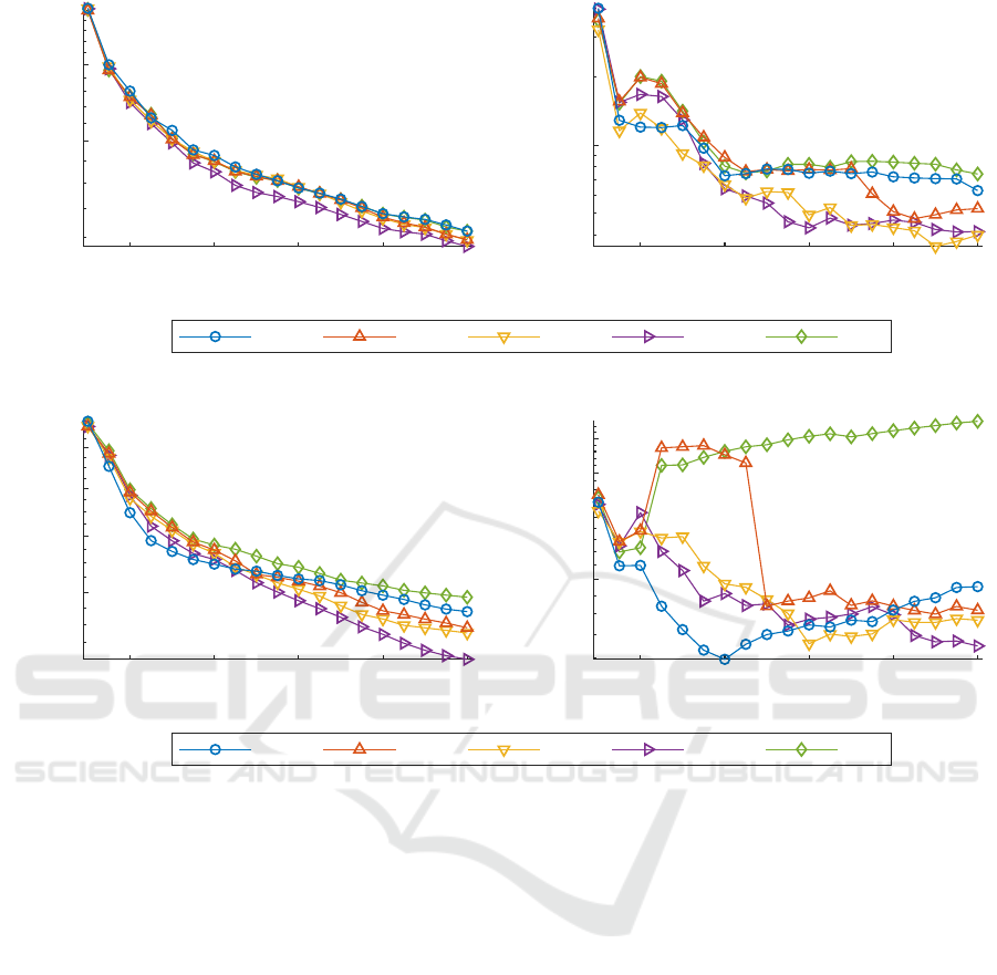
Figure 2 shows the results of setup 1. When n
Meas
/
30 , the performance of the analyzed strategies are all
very similar. From that point on, the new CVH strategy
performs significantly better than all other strategies.
This includes a low standard deviation σ
NRMSE
val,Σ
.
The low σ
NRMSE
val,Σ
shows that there is not a big dif-
ference between different runs and therefore stands for
the high robustness of this method.
Table 1: Specification of the three setups. The symbol + is
indicating high complexity or noise.
setup
model type of each
toy example output
complexity noise
sigmoid + +
1 sigmoid + +
sigmoid + +
polynomial ◦ +
2 polynomial ◦ +
multiple sigmoids
combined with steps
++ +
sigmoid + ++
3 sigmoid + +
multiple sigmoids
combined with steps
++ +
The mean of CVH has the lowest end value. This dif-
ference is significant compared to the results of RR
and CVH, which have very similar means. Assum-
ing that we want to quit our experiment at any time,
CVH should be preferred. RR and SQ have similar
mean performance, but RR inherits a lower standard
deviation and is therefore more robust. Compared to
the NRMSE
val
,Σ
of SF after n
Meas
= 100 , RR and SQ
reduce the number of points by 5 % whereas CVH re-
duces the number of points even further by 15 %. The
mean performance of G is comparable to SF. However,
the variance of G is higher, which ranks the perfor-
mance of SF over G.
Figure 3 shows that the difference between active
learning strategies is especially high in setup 2 com-
pared to the SF design. In contrast to the previous
setup, one process output has a much higher complex-
ity than the other ones. This combination shows the
benefits of CVH very clearly. When n
Meas
' 45 , CVH
performs better than all other strategies. G performs
significantly worse than the other strategies. This is
unlike the third hypothesis in section 4. Depending on
the application and the chosen strategy, it is not always
beneficial to use active learning. After n
Meas
= 100 ,
RR and SQ have no significant difference in results.
However, the standard deviation of SQ is higher dur-
ing the runs, especially for n
Meas
/ 45 . The authors
assume that the influence of the process output order
plays a role in that. Compared to that, RR shows a
more robust behavior. RR reaches the end value of
SF at n
Meas
= 75 . The standard deviations of RR and
CVH are both on similar levels. The CVH performs
significantly better than all other strategies in this sce-
nario. It reduces the number of measurement points
of a SF by 30 % and reaches the end value of RR after
n
Meas
= 80.
ICPRAM 2021 - 10th International Conference on Pattern Recognition Applications and Methods
154

SF SQ RR CVH G
n
Meas
in -
σ
NRMSE
val,Σ
in -
n
Meas
in -
µ
NRMSE
val,Σ
in -
20 40 60 80 100 20 40 60 80 100
0.1
0.15
0.2
10
−2
Figure 2: Mean µ and standard deviation σ of the NRMSE
val,Σ
of setup 1 over the number of measurements n
Meas
.
SF SQ RR CVH G
n
Meas
in -
σ
NRMSE
val,Σ
in -
n
Meas
in -
µ
NRMSE
val,Σ
in -
20 40 60 80 100 20 40 60 80 100
0.1
0.12
0.14
0.16
0.01
0.015
0.02
0.025
Figure 3: Mean µ and standard deviation σ of the NRMSE
val,Σ
of setup 2 over the number of measurements n
Meas
.
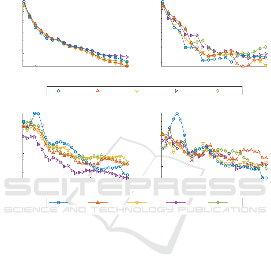
Figure 4 shows the results of setup 3. Those results
match the expectations that CVH performs worse in an
environment where a process output with high noise
and a complex one exist. For n
Meas
/ 80 , the overall
performance of CVH is not much worse than other
strategies. However, all other strategies have a better
end value. In this setup, where there is one very noisy
and one very complex process output, RR and SQ
perform best. They outperform SF at n
Meas
= 85 and
CVH already at n
Meas
= 75 . Compared to SQ, RR is
rather robust in the beginning and in the end.
The experiments confirm the hypotheses stated in
section 4. Only the third hypothesis turned out not to
be true in all cases: SF can outperform active learning
in some cases.
5.2 Benchmark Dataset
As stated in section 3, applications of active learning in
the domain of drivability calibration are rather unique
concerning the conditions and goals of other existing
tasks. That is, why there is no benchmark dataset
that fully suits the needs of an example. However we
wanted to demonstrate the practical use of such a learn-
ing strategy. This is why the jura dataset (Goovaerts,
1997), which is actually a dataset from the domain of
geostatistics, is used as a benchmark dataset here. This
dataset contains the concentration of 7 heavy metal
concentrations at different locations in the Swiss Jura.
It is the best fitting dataset, which is also used to eval-
uate the learning algorithms in (Zhang et al., 2016). In
contrast to that publication, we set the goal to model
every of the three chosen outputs equally well. Three
concentrations (Ni, Cd, Zn) are modeled as a function
of the locations during every test run. The results of
the AOS strategies presented in section 4 are averaged
over 50 test runs.
Figure 5 shows the results of the benchmark dataset.
In the beginning, SF performs significantly worse than
CVH. After n
Meas
' 100 , there are no significant dif-
ferences between those two strategies. CVH and SF
outperform G, SQ and RR in the end. Throughout
all measurements however, the mean of CVH is the
lowest. Since experiments on a test bench might be
Active Output Selection Strategies for Multiple Learning Regression Models
155

SF SQ RR CVH G
n
Meas
in -
σ
NRMSE
val,Σ
in -
n
Meas
in -
µ
NRMSE
val,Σ
in -
20 40 60 80 10020 40 60 80 100
0.01
0.015
0.02
0.025
0.12
0.14
0.16
0.18
0.2
0.22
Figure 4: Mean µ and standard deviation σ of the NRMSE
val,Σ
of setup 3 over the number of measurements n
Meas
.
SF SQ RR
CVH G
n
Meas
in -
σ
NRMSE
val,Σ
in -
n
Meas
in -
µ
NRMSE
val,Σ
in -
50 100 150 50 100 150
0.25
0.26
0.27
0.28
0.01
0.02
0.03
Figure 5: Mean µ and standard deviation σ of the NRMSE
val,Σ
of the Jura Dataset over the number of measurements n
Meas
.
stopped after any fixed number of measurements, the
results indicate that CVH is preferably used, although
it is not significantly better than SF regarding the final
model accuracy.
6 CONCLUSION
In this paper, active output selection, a new task for
active learning is introduced. It is characterized by
identifying models of multiple process outputs with
the same input dimensions. We present a new strategy
(CVH) to define the leading models in an active output
selection setup. The decision is based on the cross-
validation errors of the identified models. The paper
thoroughly analyzes the advantages and disadvantages
of said strategy. The process outputs are identified
using gaussian processes (GP). A simple maximum
variance algorithm is chosen as active learning strategy
for each individual output. The strategy is analyzed on
different toy examples, which include noisy generic
process outputs. The results of CVH are compared
against three existing learning strategies: round-robin,
sequential and global. Furthermore a passive, sequen-
tial space-filling strategy is chosen as baseline for the
active learning strategies.
The results show that the presented strategy is
preferably used in most real-world setups. The per-
formance and robustness are good compared to other
multi-output strategies. Compared to the baseline strat-
egy, CVH saves up to 30 % of the measurements. In
this setup, which has one process output with higher
complexity, CVH outperforms any other active output
selection strategy. In the particular case of a setup with
one output with high noise and one output with high
complexity, other strategies perform better than CVH.
The consideration of the estimated generalization error
could further improve the performance of CVH espe-
cially for those setups and will therefore be context to
further investigation.
The results of a benchmark dataset confirm the
good performance of CVH in the toy examples. Due
to the lack of a more suitable public benchmark dataset
ICPRAM 2021 - 10th International Conference on Pattern Recognition Applications and Methods
156

however, a geostatistics example was chosen. A public
benchmark dataset from the field of drivablity calibra-
tion would facilitate comparisons and simplify further
work on the subject. Another future research will apply
the presented strategy to setups with different numbers
of input dimensions. Moreover the application of those
strategies on different modeling and single model ac-
tive learning approaches is promising.
REFERENCES
Belz, J. and Nelles, O. (2015). Proposal for a function gener-
ator and extrapolation analysis. In 2015 International
Symposium on Innovations in Intelligent SysTems and
Applications (INISTA). IEEE.
Cai, W., Zhang, M., and Zhang, Y. (2017). Batch Mode
Active Learning for Regression With Expected Model
Change. IEEE Transactions on Neural Networks and
Learning Systems.
Cai, W., Zhang, Y., and Zhou, J. (2013). Maximizing Ex-
pected Model Change for Active Learning in Regres-
sion. In 2013 IEEE 13th International Conference on
Data Mining, Dallas, TX, USA. IEEE.
Cohn, D. A. (1996). Neural Network Exploration Using
Optimal Experiment Design. Neural Networks.
Dursun, Y., Kirschbaum, F., Jakobi, R., Gebhardt, A., Goos,
J.-C., and Rinderknecht, S. (2015). Ansatz zur adap-
tiven Versuchsplanung für die Längsdynamikapplika-
tion von Fahrzeugen auf Prüfständen. In 6. Interna-
tionales Symposium für Entwicklungsmethodik.
Goovaerts, P. (1997). Geostatistics for natural resources
evaluation. Oxford University Press on Demand.
Hartmann, B. and Nelles, O. (2013). Adaptive Test Planning
for the Calibration of Combustion Engines – Method-
ology. Design of Experiments (DoE) in Engine Devel-
opment.
Klein, P., Kirschbaum, F., Hartmann, B., Bogachik, Y., and
Nelles, O. (2013). Adaptive Test Planning for the Cali-
bration of Combustion Engines – Application. Design
of Experiments (DoE) in Engine Development.
MacKay, D. J. C. (1992). Information-Based Objective Func-
tions for Active Data Selection. Neural Computation.
Park, S. H. and Kim, S. B. (2020). Robust expected model
change for active learning in regression. Applied Intel-
ligence.
Pasolli, E. and Melgani, F. (2011). Gaussian process re-
gression within an active learning scheme. In 2011
IEEE International Geoscience and Remote Sensing
Symposium, Vancouver, BC, Canada. IEEE.
Rasmussen, C. E. and Williams, C. K. I. (2008). Gaussian
processes for machine learning. MIT Press, Cam-
bridge, Mass., 3. print edition.
Seo, S., Wallat, M., Graepel, T., and Obermayer, K. (2000).
Gaussian Process Regression: Active Data Selection
and Test Point Rejection. In Mustererkennung 2000.
Springer Berlin Heidelberg, Berlin, Heidelberg.
Settles, B. (2009). Active Learning Literature Survey. Tech-
nical report, University of Wisconsin–Madison.
Sugiyama, M. and Rubens, N. (2008). Active Learning with
Model Selection in Linear Regression. In Proceedings
of the 2008 SIAM International Conference on Data
Mining. Society for Industrial and Applied Mathemat-
ics.
Tietze, N. (2015). Model-based Calibration of Engine Con-
trol Units Using Gaussian Process Regression. PhD
thesis, Technische Universität Darmstadt, Darmstadt.
Zhang, Y., Hoang, T. N., Low, K. H., and Kankanhalli, M.
(2016). Near-optimal active learning of multi-output
Gaussian processes. In Thirtieth AAAI Conference on
Artificial Intelligence.
Active Output Selection Strategies for Multiple Learning Regression Models
157