State Tracking in the Presence of Heavy-tailed Observations

Yaman Kindap

Department of Computer Engineering, Bogazici University, Bebek, Istanbul, Turkey

Keywords:

Signal Processing, Bayesian Models, Stochastic Methods, Classiﬁcation, Clustering.

Abstract:

In this paper, we deﬁne a state-space model with discrete latent states and a multivariate heavy-tailed observa-

tion density for applications in tracking the state of a system with observations including extreme deviations

from the median. We use a Gaussian distribution with an unknown variance parameter which has a Gamma

distribution prior depending on the state of the system to model the observation density. The key contribution

of the paper is the theoretical formulation of such a state-space model which makes use of scale mixtures

of Gaussians to yield an exact inference method. We derive the framework for estimation of the states and

how to estimate the parameters of the model. We demonstrate the performance of the model on synthetically

generated data sets.

1 INTRODUCTION

Modelling sequential data and making inference on

these systems is an essential area of research in vari-

ous ﬁelds of science and engineering. Sequential data

may arise from dynamical systems in the form of a

time series or a single dimensional spatial process

where the position of an observation is critical such

as in biological sequences. While the evolution of a

dynamical system is often described by a determin-

istic function, some systems are inherently stochastic

or the complexity of some systems may require statis-

tical arguments in which case the model of the system

evolution is stochastic.

While randomness caused by measurement noise

is involved in most systems of interest, the evolu-

tion of the dynamical system may be stationary which

simply means that some statistical properties of the

system are constant with respect to time. Such sys-

tems can be modelled by evolution functions that

are independent of time. On the other hand, non-

stationary dynamical systems present the additional

problem that the evolution mechanism of the system

also changes in time. In such systems, one solution is

to cluster the observations in terms of similar char-

acteristic behaviour in order to model the different

dynamics of the system separately. One extensively

studied model that is used for this problem is the hid-

den Markov model with a mixture of Gaussian ob-

servation likelihoods (GHMM) (Rabiner, 1990). Be-

https://orcid.org/0000-0002-9269-039X

cause of its mathematical simplicity and its ability to

estimate any density, the GHMM can be used in vari-

ous different applications.

However, for systems that display extreme devia-

tions from its median characteristic behavior for each

state, the GHMM is limited because of its assump-

tion that observations follow a conditional Gaussian

distribution. In this work, we show how to expand

the GHMM in a concise mathematical way by intro-

ducing an additional latent scale parameter into the

GHMM which enables the dynamical modeling of

heavy-tailed observations. Algorithms for inference

of latent variables and learning the parameters of the

proposed model are presented along with their theo-

retical formulations.

The use of scale mixture of Gaussian distribu-

tions for the purpose of modelling heavy-tailed ob-

servations is presented in (Cemgil et al., 2007). Re-

cently, the extension of hidden Markov models to

include heavy-tailed observations are studied, espe-

cially in the case of Student’s t-distribution (Chatzis

et al., 2009). It has been shown that the Student’s t-

distribution HMM (SHMM) is able to identify more

persistent states in time series data (Bulla, 2011). The

use of SHMMs in classiﬁcation tasks is presented in

(Zhang et al., 2013).

Hidden Markov models used in the literature with

t-distribution as the emission distribution (SHMM)

use the well-known derivation of t-distribution as a

scale mixture of the Gaussian distribution where the

variance of the Gaussian distribution is treated as a

Kindap, Y.

State Tracking in the Presence of Heavy-tailed Observations.

DOI: 10.5220/0010150601350142

In Proceedings of the 10th International Conference on Pattern Recognition Applications and Methods (ICPRAM 2021), pages 135-142

ISBN: 978-989-758-486-2

135

random variable. While this formulation allows the

expectation-maximization algorithm to be tractable,

the main simplicity of its derivation comes from the

fact that the resulting distribution has an exponen-

tial family form, which there is no reference to in the

HMM literature. In this work we explicitly show this

derivation. Furthermore, rather than introducing the

variance of the Gaussian distribution into the model

as a latent variable, previous works only use this for-

mulation for mathematical convenience. In this work,

we will treat the variance of the Gaussian distribution

as an additional latent variable in our model which al-

lows us to have a dynamically scaled model at each

time step.

2 GAUSSIAN-GAMMA HIDDEN

MARKOV MODEL

Figure 1: Probabilistic graphical model of GGHMM.

The Gaussian-Gamma hidden Markov model

(GGHMM) is a particular class of the state-space

model shown in Figure 1 where the variables x

1:T

are

discrete-valued while w

1:T

and y

1:T

are continuous-

valued. Additionally, observed variables are shaded

for emphasis. The model assumes that an unobserved

ﬁrst-order Markov process generates observations

from a mixture distribution p(y

). Hence, the

HMM can be interpreted as an extension of mixture

models where sequential information is also encoded

(Bishop, 2006).

Let’s assume that we have a N-state system. The

state at time t, deﬁned as x

, has an evolution pro-

cess which is assumed to be a discrete state, discrete

time ﬁrst order Markov process. Thus, we can rep-

resent this process as a categorical distribution where

the parameters of the distribution depend on the value

assumed by the previous state x

t−1

f (x

t−1

,A) =

∏

i=1

∏

j=1

t−1

=i][x

= j]

i j

(1)

where a

i j

is the i

row and j

column of a transi-

tion matrix A. The notation [P] is the Iverson bracket

where [P] equals 1 if P is true and 0 otherwise. The

initial probabilities of states at time 1 is parameterized

as a vector π, where the density is deﬁned as p(x

|π).

An observation at time t, deﬁned as y

, is assumed

to be conditionally independent of previous observa-

tions y

1:t−1

given the current state x

and has a k-

dimensional Gaussian distribution with mean µ and

an unknown variance. We treat the variance of the ob-

servation process as a random variable and therefore

deﬁne a scaling random variable w

that has a Gamma

distribution with parameters α = β =

. Similar to the

state x

of the system, the scaling variable w

is a la-

tent variable. Furthermore, we assume that the value

of parameters of our model depends on the current

state of the system. The corresponding model can be

shown as:

,ν ∼ Gamma





(

)

Γ(

)

−1

exp



−





(2)

d(y

,µ) = (y

− µ)

−1

− µ) (3)

,µ,Σ ∼ Gaussian



µ,



(2π)

|Σ|

exp



−

d(y

,µ)



(4)

where Σ is considered to be a constant covariance pa-

rameter of the observation density encoding the cor-

relations between different observations and d(y

,µ)

is a distance measure. The scale of the covariance

parameter is adjusted according to w

. When x

= i

the state dependent parameters are shown with the

subscript i as µ

, Σ

and ν

. This parameterization is

equivalent to setting a conjugate prior on the variance

of the Gaussian distribution. Such a formulation of

the observation variable y

has the convenient prop-

erty that when we integrate over the latent scale vari-

able w

of the Gaussian distribution it becomes a gen-

eralized multivariate t-distribution which has a den-

sity shown in equation 5 where C is the normaliza-

tion constant shown in equation 6. Furthermore, the

Gaussian-Gamma distribution density deﬁne an expo-

nential family which enable efﬁcient inference.

p(y

,µ,Σ, ν) = C



1 +

d(y

,µ)



−

ν+k

(5)

C =

Γ(

ν+k

)

Γ(

)ν

(k/2)

|Σ|

(1/2)

(6)

ICPRAM 2021 - 10th International Conference on Pattern Recognition Applications and Methods

136

Using the model assumptions we have deﬁned,

the joint probability distribution of the variables y

1:T

and x

1:T

is deﬁned as:

p(y

1:T

|θ) = p(x

|π)

∏

t=2

p(x

t−1

,A)

∏

t=1

p(y

,µ,Σ)p(w

,ν)

(7)

where θ is the set of parameters of the model.

3 LATENT VARIABLE

INFERENCE

Our main goal is to infer the posterior probability dis-

tribution of the state of the system at each time t. As-

suming that our model sufﬁciently represents the sys-

tem and the true parameters of the model are known,

the posterior probability of x

can be calculated with-

out knowing the posterior distribution of w

since we

will be marginalizing it out. However, for a complete

understanding of the model and it’s requirement in pa-

rameter estimation, we will also be concerned with

the inference of the posterior distribution of w

We formulate the ﬁltering and smoothing prob-

lems for the estimation of latent variables in our

model using a recursive Bayesian framework. In the

GGHMM the ﬁltered density includes w

and shown

as p(x

1:t

,θ). Similarly the smoothed density is

deﬁned as p(x

1:T

,θ).

3.1 Filtering

Let’s assume that the posterior distribution of the state

t−1

at time t − 1 is known. Using the state evolution

equation f (x

t−1

,A) we can obtain a prior distribu-

tion on the state x

p(x

1:t−1

,θ) =

∑

t−1

f (x

t−1

,A)p(x

t−1

1:t−1

,θ)

(8)

The joint posterior distribution on the latent vari-

ables x

and w

is shown in equation 9.

p(x

1:t

,θ) =

p(y

1:t−1

,θ)

∗

p(y

,µ,Σ)p(w

,ν)p(x

1:t−1

,θ)

(9)

Notice that the denominator p(y

1:t−1

,θ) is ob-

tained by marginalizing x

and w

out from the nom-

inator in equation 9. At this point, we can obtain

the posterior distribution of x

by using the convenient

property of integrating out w

in order to obtain the

density of t-distribution.

p(x

1:t

,θ) =

p(y

,µ,Σ, ν)p(x

1:t−1

,θ)

p(y

1:t−1

,θ)

(10)

where the density p(y

,µ,Σ, ν) is the generalized t-

distribution shown in equation 5. Notice that using

the chain rule, the posterior distribution of the latent

variables can be factorized as shown in equation 11.

p(x

1:t

,θ) = p(x

1:t

,θ)p(w

1:t

,θ) (11)

Using the factorization shown in equation 11, the

ﬁltered posterior distribution of w

can be obtained

using equation 12.

p(w

1:t

,θ) =

p(x

1:t−1

,θ)

∗

p(y

,µ,Σ)p(w

,ν)p(x

1:t−1

,θ)

(12)

where the joint density p(x

1:t−1

,θ) is equiv-

alent to the nominator of equation 10. With

some rearrangement of parameters, the joint density

p(w

1:t

,θ) actually deﬁnes an exponential family

in equation 12. This property enables us to have some

very efﬁcient algorithms.

p(w

1:t

,θ) =

−2+k

exp



−

d(y

,µ)w



Γ(

)



d(y

,µ)+



−

(13)

3.1.1 Moments of the Latent Scaling Variable

Since we will be needing to calculate some functions

of w

in the parameter learning section, let’s analyze

the posterior distribution of w

shown in equation 13.

Firstly, notice that the only information we have about

is through the observation of y

and the estimate of

. Any observation other than y

does not have any

inﬂuence over our estimates of w

. While we expect

that consecutive w

values do not vary signiﬁcantly

in real data sets, the GGHMM model does not take

this dependence into account in order to simplify the

mathematical formulation of the model. This assump-

tion mathematically means that we cannot improve

our estimate of the posterior distribution by using a

State Tracking in the Presence of Heavy-tailed Observations

137

smoothing procedure and p(w

= i,y

1:t

,θ) is equal

to p(w

= i,y

1:T

,θ). We will comment on this lim-

itation of our model in section 6.

Let’s now calculate the moments of the sufﬁcient

statistics of w

deﬁned by equation 13. For expo-

nential families, we deﬁne the functions t(x), η(θ)

and a(η). We have 2-dimensional sufﬁcient statistics

shown as:

) = −w

) = log(w

)

(14)

The parameters η(θ) corresponding to these sufﬁ-

cient statistics are:

(θ) =

d(y

,µ)+

(θ) =



− 2 + k



(15)

Most importantly the log-normalizer function

a(η) is deﬁned as:

a(η) = log





d(y

,µ)+



−(

)

Γ(

+ k

)



= log



−(η

+1)

Γ(η

+ 1)



(16)

Now, using the log-normalizer function, we can

calculate the ﬁrst moments of the sufﬁcient statistics

−w

and log(w

∂

∂η

a(η) =

Γ(η

+ 1)(−1)(η

+ 1)η

−(η

+2)

−(η

+1)

Γ(η

+ 1)

= (−1)(η

+ 1)η

−1

= E(−w

)

(17)

We can transform the parameters η

and η

into

their θ forms in order to obtain an expression for the

expectation of w

∂

∂η

a(η) = (−1)



+ k

h

d(y

,µ)+

−1

= E(−w

)

(18)

Since the expectation operator scales linearly

when multiplied by a constant factor, we ﬁnd that:

E(w

) =



+ k

h

d(y

,µ)+

−1

(19)

Similarly, let’s ﬁnd the ﬁrst moment of log(w

∂

∂η

a(η) = ψ

(η

) − ln(η

)

(20)

where the function ψ

(z) is the digamma function

which describes the derivative of the Gamma function

Γ(z) through the identity:

(z) = Γ(z)ψ

(z) (21)

We can transform the parameters η

and η

into

their θ forms in order to obtain an expression for the

expectation of log(w

∂

∂η

a(η) = ψ

(η

) − ln(η

)

= ψ



+ k



− ln



d(y

,µ)+



(22)



log(w

)



= ψ



+ k



−ln



d(y

,µ)+



(23)

3.2 Smoothing

In this section, our goal is to obtain a smoothed esti-

mate of the latent variables x

1:T

which utilizes the full

information available at time T . As we have men-

tioned, the smoothed posterior density of w

is equal

to the ﬁltered posterior since we do not have any se-

quential dependence between consecutive w

values.

The smoothed estimate we aim to calculate in this sec-

tion is deﬁned as p(x

1:T

,θ).

Notice that similar to our considerations in an

HMM, we can use the ﬁltered estimates p(x

i,y

1:t

|θ) together with a density p(y

t+1:T

= i, θ) in

order to calculate the joint probability density of the

model:

p(x

1:T

|θ) = p(x

1:t

|θ)p(y

t+1:T

,θ) (24)

which can be normalized by using the incomplete data

likelihood p(y

1:T

|θ) in order to obtain the smoothed

estimate p(x

1:T

,θ).

Assuming we know p(y

t+1:T

,θ), we can ﬁnd a

joint distribution p(y

t:T

t−1

,θ) by initially using the

emission density p(y

,µ,Σ, ν) of the multivariate t-

distribution in order to ﬁnd the likelihood of y

t:T

for

each state x

. We call this operation the update step

since it involves the addition of an observation y

to a

known joint probability distribution.

p(y

t:T

,θ) = p(y

,µ,Σ, ν)p(y

t+1:T

,θ) (25)

ICPRAM 2021 - 10th International Conference on Pattern Recognition Applications and Methods

138

The next step is to estimate the likelihood of y

t:T

given that we only know state x

t−1

. This estimate

can be obtained by a marginalization procedure and

is called postdiction since it involves the estimation

of the likelihood of a state with information from the

future.

p(y

t:T

t−1

,θ) =

∑

p(y

t:T

,θ) f (x

t−1

,A) (26)

4 PARAMETER LEARNING

We formulate a maximum likelihood estimation pro-

cedure for our model based on the expectation-

maximization algorithm. The well known Baum-

Welch algorithm is derived for the hidden Markov

model which has the same state transition structure

as our model. Thus, we build upon this algorithm to

derive update equations for the model parameters µ, Σ

and ν, and note that π and A are same the same as in

the Baum-Welch algorithm (Bilmes, 2000). The max-

imum likelihood estimation problem can be stated as:

∗

= argmax

log p(y

1:T

|θ) (27)

The expectation maximization algorithm is a

method of maximizing equation 27 in an itera-

tive manner. Using Jensen’s inequality we can ﬁnd

a lower bound to the incomplete data likelihood

p(y

1:T

|θ) and maximize this lower bound at each iter-

ation. The lower bound turns out to be in the form of

an expectation over the posterior distribution of the

latent variables x

1:T

and w

1:T

, p(x

1:T

,θ),

which is shown in equation 28.

log p(y

1:T

|θ) ≥ E



log

p(y

1:T

|θ)

p(x

1:T

,θ)



(28)

Let’s deﬁne the estimated parameters at each iter-

ation with a superscript k, shown as θ

(k)

. For compu-

tational efﬁciency, the posterior distribution over the

latent variables are calculated with the set of parame-

ters θ

(k)

. The details of this derivation is similar to the

considerations in the Baum-Welch algorithm which

are shown in detail in (Bilmes, 2000). In summary, it

is based on the chain rule of probability applied to the

posterior distribution of the latent variables.

In order to simplify the update equations we de-

ﬁne the posterior probability distribution of x

, p(x

i|y

1:T

,θ

(k)

), as γ

(k)

(i), which is consistent with the lit-

erature. The update equations for µ

and Σ

are shown

below:

(k+1)

∑

t=1

(k)

(i)

t,i

∑

t=1

(k)

(i)

t,i

(29)

(k+1)

∑

t=1

(k)

(i)

t,i

− µ

(k+1)

)(y

− µ

(k+1)

)

∑

t=1

(k)

(i)

t,i

(30)

where we denote the posterior expected value of w

t,i

for brevity. Notice that we have shown the

calculation of this expectation is relatively simple be-

cause of the exponential family form of the posterior

distribution of w

t,i

shown in 3.1.1. Therefore, equa-

tions 29 and 30 have similar analogs in Baum-Welch

update equations, and their calculation is straightfor-

ward.

Unfortunately, the update equation for ν

does not

have a simple form similar to equations 29 and 30

because of the presence of the Gamma function Γ(z)

in the gamma distribution p(w

= i,ν). We have

to introduce the digamma function ψ

(z) which is

deﬁned as the logarithmic derivative of the gamma

function. Let’s deﬁne the posterior distribution of w

p(w

= i,y

1:T

,θ

(k)

), as κ

(k)

. Taking the derivative

of the expectation shown in equation 28 with respect

to ν

and setting it equal to zero yields:

0 = log





+ 1 − ψ





+ K (31)

where K denotes a constant with respect to ν

and can

be shown as:

K =

∑

t=1

(k)

(i)

∞

(k)



log(w

t,i

) − w

t,i



∑

t=1

(k)

(i)

(32)

Notice that the nominator of the equation above

includes the expected value of log(w

) and w

which

we previously calculated in section 3.1.1.

In order to ﬁnd a value ν

(k+1)

, we propose to

ﬁnd the root of the equation 31 by using the bisec-

tion (binary search) method. We prefer this method

over other root ﬁnding algorithms such as the New-

ton–Raphson method because it enables us to con-

strain the space of possible ν

values to be in (1,∞).

This is important for the robustness of the parameter

estimation process since the student’s t-distribution is

only deﬁned for ν > 0 and its mean is deﬁned for

ν > 1. When the mean of the emission density is not

deﬁned, all other parameters diverge. An alternative

method of approximating the value of ν

(k+1)

is shown

in (Shoham, 2002).

State Tracking in the Presence of Heavy-tailed Observations

139

5 EXPERIMENTS

In this section, we test the performance of our pro-

posed Gaussian-Gamma hidden Markov model with

synthetically generated data since that is the only case

we can know the actual realizations of the latent vari-

ables. Problems involving real data in the context

where we assume the presence of latent variables gen-

erally requires the construction of objective functions

which heavily inﬂuence the performance of such a

model and is out of scope of this work.

We present the theoretical capabilities of our

model by evaluating its performance on state identiﬁ-

cation for synthetically generated multivariate heavy-

tailed time series data and compare it to a Gaussian

hidden Markov model. The synthetic data genera-

tion process of a multivariate heavy-tailed time series

involves a state-space model with an identical struc-

ture to the GGHMM. The parameters of the model

are randomly generated in each realization of the ex-

periment with a 2-dimensional latent Markovian state

space. Our aim is to understand the effects of max-

imum training epochs used for each realization and

dimensionality of the observation space on the state

identiﬁcation task using smoothed estimates of the la-

tent states.

5.1 Evaluation Criteria

There are various evaluation criteria for classiﬁcation

and clustering tasks such as accuracy, precision and

recall. However, we need to consider the underlying

decision making problem in order to select an appro-

priate metric. While our main goal is to identify the

state at each time t, since we assume that states are

persistent in a dynamical system, the difﬁculty of this

task arise from state change-points.

Let’s discuss the potential effectiveness of each

evaluation metric in order to understand their signiﬁ-

cance. Accuracy, deﬁned in equation ??, measures the

correctness of all state identiﬁcations. This measure

does not reﬂect the persistent nature of our dynamical

system since correctly guessing that there wasn’t any

change in the system is not as informative as detecting

a change.

(33)

Accuracy =

∑

True Positive +

∑

True Negative

∑

Total Population

Instead of focusing on identifying every state, let’s

direct our attention to how well we can identify a

speciﬁc state. This change in our focus leads us to

the precision and recall metrics which are deﬁned

in equations 34 and 35, respectively. Precision is a

measure of the correctness of our positively identi-

ﬁed states and recall is a measure of how correct we

were actually able to identify a speciﬁc state in reality.

These two metrics are a better measure of the perfor-

mance of our models considering that states of a sys-

tem are not equally informative such as in the case of

identifying malignant and benign biological activities.

Thus, we select the state with higher overall standard

deviations as the relevant state to be identiﬁed, since

we assume that critical states have higher uncertainty.

We report the corresponding precision and recall val-

ues for each realization of the experiment.

Precision =

∑

True Positive

∑

True Positive +

∑

False Positive

(34)

Recall =

∑

True Positive

∑

Condition Positive

(35)

Since we do not want our models to be dependent

on a speciﬁc data set, we generate multiple different

realization of the experiments with randomly gener-

ated data sets and compare the models based on an

equally weighted average performance on these dif-

ferent realizations. The results report the mean and

standard deviation in each evaluation criteria.

5.2 Performance Statistics of

Experiments

The performance of both models highly depend on

the random data generation mechanism. Particularly,

having a heavy-tailed distribution only matters in the

case where the theoretical probability distribution of

each state intersects. This fact is actually quite intu-

itive when we consider the one-dimensional observa-

tion space case. If the two states have mutually exclu-

sive probability distributions it would be easy to dis-

tinguish between the two. The problem gets progres-

sively more difﬁcult as their sample space intersect.

Thus, we constrain the mean behavior of both states

to be close in terms of some dispersion metric. This

corresponds to a unique problem where the regimes of

the process have very similar average behavior while

the covariance structure and the extreme events de-

ﬁne their difference. In order to reﬂect the persistence

of each state while still keeping the structure of data

relatively random, the diagonal terms in the transition

matrix are constrained to be a

≥ 0.8. We explore the

performance of each model according to this case and

a particular realization of the synthetically generated

data is shown in Figure 2 where different states are

shaded.

ICPRAM 2021 - 10th International Conference on Pattern Recognition Applications and Methods

140

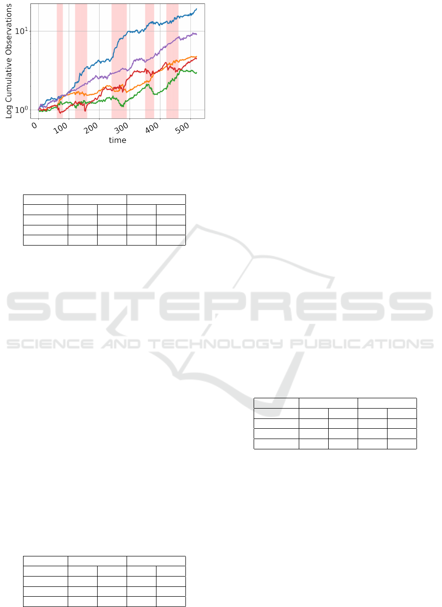
Figure 2: Example realization of experiments.

Table 1: Performance statistics of equally trained models.

GGHMM GHMM

Mean Std Mean Std

Accuracy 0.849 0.150 0.907 0.145

Precision 0.782 0.126 0.831 0.171

Recall 0.727 0.131 0.911 0.207

Initially, we have recorded the results of 100 dif-

ferent realizations of the experiment where both of the

models are trained for a maximum of 20 epochs. The

observation space is 3-dimensional and each realiza-

tion has a length of 500. The results are presented

in Table 1. We see that the GHMM has a signiﬁ-

cantly better performance in terms of mean accuracy

and standard deviation in accuracy throughout the re-

alizations. The same result carries over to their perfor-

mance in terms of precision and recall. Thus, under

the current conditions the GHMM is a better choice.

We arguably need to train the GGHMM model

with more maximum training epochs in order have

comparable performance statistics because of its in-

creased complexity. It is likely that the parameters did

not converge to a set which maximizes the likelihood

of the incomplete data set in 20 epochs. The con-

vergence properties of the EM algorithm for the case

of Gaussian emissions are studied in (Xu and Jordan,

1996). Since the GHMM is relatively simpler when

compared to the GGHMM, we conclude that under

constrained compute power the GHMM displays bet-

ter results.

Table 2: Performance statistics of unconstrained training

epoch realizations.

GGHMM GHMM

Mean Std Mean Std

Accuracy 0.957 0.063 0.901 0.139

Precision 0.953 0.099 0.868 0.241

Recall 0.948 0.116 0.896 0.218

Let’s investigate the effects of maximum training

epochs in the performance statistics of both models.

We have recorded the results of 100 different realiza-

tion of the experiment where the GGHMM is trained

until its results converge according to a threshold dif-

ference between each iteration and the GHMM is

trained for a maximum of 20 epochs. The results are

shown in Table 2. Since we left the maximum train-

ing epochs for the GHMM unchanged, we expect that

the mean and standard deviation in performance mea-

sures are not signiﬁcantly different from the ﬁrst set

of 100 realizations. Results show that we can make a

signiﬁcant improvement for the GGHMM by increas-

ing the maximum training epochs. The GGHMM has

a better performance in every metric compared to both

the GHMM for these realizations and the GGHMM

for the previous 100 realizations. Furthermore, con-

vergence in the GGHMM is reached in 80 epochs on

average.

However, considering that a single epoch of train-

ing in GGHMM is signiﬁcantly longer than a single

epoch in GHMM because of the increased complex-

ity of the calculations, both models may have their

advantages. For most problems, the training time of

the model is another important selection metric be-

cause of time constraints. While the GGHMM is able

to display better performance, it is at the cost of sig-

niﬁcantly more training time. The assessment of how

this fact affects the choice between the two models

is dependent on the problem and the priorities of the

researcher.

Table 3: Performance statistics in 5-dimensional observa-

tion space.

GGHMM GHMM

Mean Std Mean Std

Accuracy 0.957 0.073 0.867 0.156

Precision 0.941 0.100 0.893 0.179

Recall 0.961 0.057 0.880 0.227

Next, we investigate the effects of the dimen-

sionality of the observation space. Thus, we have

recorded the results of 100 different realizations of

the experiment with a 2-dimensional latent Marko-

vian state-space, a 5-dimensional observation space

and each realization has a length of 500. As we have

established in the previous 200 realizations of the ex-

periment, a better performance is recorded for the

GGHMM when we let the model train until conver-

gence. Since the average epochs for GGHMM was

found to be 80 for convergence, we use this value as

an upper bound to constrain the experiment. There-

fore, we train the GHMM and GGHMM for a maxi-

mum of 20 and 80 training epochs, respectively. The

State Tracking in the Presence of Heavy-tailed Observations

141

results are shown in Table 3. Notice that we can-

not show any improvement in the performance for

the GHMM while the performance of the GGHMM

is similarly good compared to the 3 dimensional case.

Thus, we conclude that the dimensions of the obser-

vation space does not have a signiﬁcant effect on the

performance for these realizations.

Overall, we are able to show that the GGHMM

performs better than the GHMM under speciﬁc cir-

cumstances. While both models have their advan-

tages, there may be some beneﬁt in using a GGHMM

for the identiﬁcation of states of a system with ex-

tereme deviations over the GHMM. On the other

hand, the increased training time for the GGHMM

also needs to be considered when deploying such a

model in production.

6 CONCLUSION

In this work, we have introduced an extension to the

hidden Markov model in order to identify the states

of a non-stationary dynamical system with observa-

tions that have heavy-tailed distributions. Such sys-

tems pose a signiﬁcant challenge to researchers in

computational ﬁelds and even incremental advance-

ments may be highly lucrative.

Our proposed model, the Gaussian-Gamma hid-

den Markov model, can be considered as a variant

of the hidden Markov model where we increase the

complexity of the model in order to accommodate our

prior knowledge on heavy-tailed distributions. The

increased complexity of our model can be efﬁciently

handled by formulating the observation density as an

exponential family. Our model can potentially be

used to model various non-stationary dynamic sys-

tems with multiple regimes and heavy-tailed distri-

butions and is capable of representing heteroscedastic

processes within each state and is highly ﬂexible. Fur-

thermore, the model is mostly analytically tractable

aside from requiring an auxiliary root ﬁnding algo-

rithm. This allows it to be trained relatively quickly

compared to the state-of-the-art deep neural networks

and requires much less data in order to be trained.

We have shown the application of GGHMM in

state identiﬁcation for synthetically generated data.

Results show that the GGHMM has a performance

comparable with the GHMM in the state identiﬁca-

tion task. In terms of improvements to the GGHMM,

one obvious way of improvement can come from ex-

plicitly modelling the dependencies between the se-

quential latent scale variables. However, since this

would introduce intractable calculations we have left

it as a future research.

Another source of improvement may be to also

learn the number latent states in the system. Such

models use the hierarchical Dirichlet process as their

latent representation of the state transition system

(Teh et al., 2006). For an unknown number of states,

the intuition that the states are persistent can be mod-

elled using the work in (Fox et al., 2007). For more

efﬁcient learning in such models, practical considera-

tions are presented in (Ulker et al., 2011).

REFERENCES

Bilmes, J. (2000). A gentle tutorial of the em algorithm

and its application to parameter estimation for gaus-

sian mixture and hidden markov models. Technical

Report ICSI-TR-97-021, University of Berkeley, 4.

Bishop, C. M. (2006). Pattern Recognition and Ma-

chine Learning (Information Science and Statistics).

Springer-Verlag, Berlin, Heidelberg.

Bulla, J. (2011). Hidden markov models with t components.

increased persistence and other aspects. Quantitative

Finance, 11(3):459–475.

Cemgil, A. T., Fevotte, C., and Godsill, S. J. (2007). Vari-

ational and stochastic inference for bayesian source

separation. Digital Signal Processing, 17(5):891 –

913. Special Issue on Bayesian Source Separation.

Chatzis, S., Kosmopoulos, D., and Varvarigou, T. (2009).

Robust sequential data modeling using an outlier tol-

erant hidden markov model. IEEE transactions on

pattern analysis and machine intelligence, 31:1657–

69.

Fox, E., Sudderth, E., Jordan, M., and Willsky (2007).

The sticky hdp-hmm: Bayesian nonparametric hidden

markov models with persistent states. Technical Re-

port 2, MIT Laboratory for Information & Decision

Systems, Cambridge, MA 02139.

Rabiner, L. R. (1990). A Tutorial on Hidden Markov Mod-

els and Selected Applications in Speech Recognition,

page 267–296. Morgan Kaufmann Publishers Inc.,

San Francisco, CA, USA.

Shoham, S. (2002). Robust clustering by determinis-

tic agglomeration em of mixtures of multivariate t-

distributions. Pattern Recognition, 35:1127–1142.

Teh, Y. W., Jordan, M. I., Beal, M. J., and Blei, D. M.

(2006). Hierarchical dirichlet processes. Journal of

the American Statistical Association, 101(476):1566–

1581.

Ulker, Y., Gunsel, B., and Cemgil, A. T. (2011). An-

nealed smc samplers for nonparametric bayesian mix-

ture models. IEEE Signal Processing Letters, 18(1):3–

Xu, L. and Jordan, M. I. (1996). On convergence properties

of the em algorithm for gaussian mixtures. Neural

Comput., 8(1):129–151.

Zhang, H., Jonathan Wu, Q. M., and Nguyen, T. M. (2013).

Modiﬁed student’s t-hidden markov model for pattern

recognition and classiﬁcation. IET Signal Processing,

7(3):219–227.

ICPRAM 2021 - 10th International Conference on Pattern Recognition Applications and Methods

142