Efficient Construction of Neural Networks Lyapunov Functions with
Domain of Attraction Maximization
Benjamin Bocquillon
1
, Philippe Feyel
1
, Guillaume Sandou
2
and Pedro Rodriguez-Ayerbe
2
1
Safran Electronics & Defense, 100 avenue de Paris, Massy, France
2
L2S, CentraleSup
´
elec, CNRS, Universit
´
e Paris-Saclay, 3 rue Joliot Curie, 91192 Gif-Sur-Yvette, France
Keywords:
Lyapunov Function, Domain of Attraction, Optimization, Neural Network, Nonlinear System.
Abstract:
This work deals with a new method for computing Lyapunov functions represented by neural networks for
autonomous nonlinear systems. Based on the Lyapunov theory and the notion of domain of attraction, we
propose an optimization method for determining a Lyapunov function modelled by a neural network while
maximizing the domain of attraction. The potential of the proposed method is demonstrated by simulation
examples.
1 INTRODUCTION
In 1892, Lyapunov introduced a way to prove stability
of mechanical nonlinear systems (Lyapunov, 1892).
He defined a scalar function inspired by a classical
energy function, which has three important properties
that are sufficient for establishing the Domain Of At-
traction (DOA) of a stable equilibrium point: (1) it
must be a local positive definite function; (2) it must
have continuous partial derivatives, and (3) its time
derivative along any state trajectory must be negative
semi-definite. While Lyapunov theory provides pow-
erful guarantees concerning equilibrium points’ sta-
bility once an appropriate function is identified, there
is no general method for constructing such a function,
call in the sequel a Lyapunov function.
Various methods to compute Lyapunov functions
have surfaced in the literature, especially with the
emergence of efficient optimization methods. At-
tempts have been made to compute the best quadratic
Lyapunov function, with (Panikhom and Sujitjorn,
2012) for example. However, these methods are too
conservative in case of industrials complex systems.
Several other computational approaches to construct
complete Lyapunov functions have been published,
for instance (Arg
´
aez et al., 2018), where the authors
present a new iterative algorithm that avoids obtain-
ing trivial solutions when constructing complete Lya-
punov functions. This algorithm is based on mesh-
free numerical approximation and analyses the fail-
ure of convergence in certain areas to determine the
chain-recurrent set. Although efficient, this method
looks like difficult to implement for real complex sys-
tems that we can find in industrial framework in which
flexibility is needed. Endless, the survey (Giesl and
Hafstein, 2015) has brought different methods and de-
scribed the state of art of the vaste variety of methods
to compute Lyapunov functions of various kinds of
systems. It proposes conservative methods when the
system is complex and highly non-linear.
However, in our opinion, the emergence of Arti-
ficial Intelligence tool such as Machine Learning and
Neural Networks seems to be a good and powerful al-
ternative for industrials to justify and then certificate
quickly complex and intelligent systems that we can
find in aero for instance. One of the first paper us-
ing Artificial Intelligence to compute Lyapunov func-
tion is (Prokhorov, 1994), where a so called Lyapunov
Machine, which is a special-design artificial neural
network, is described for Lyapunov function approx-
imation. The author indicates that the proposed algo-
rithm, the Lyapunov Machine, has substantial compu-
tational complexity among other issues to be resolved
and defers their resolution to future work. (Banks,
2002) suggests a Genetic Programming for comput-
ing Lyapunov functions. However, the Lyapunov
functions computed may have locally a conservative
behavior. We overcome all these limits using Neural
Networks. Neural Networks are widely used in a va-
riety of applications, such as in image classification
and in natural language processing. In general, neural
networks are powerful regressors, and thus lend them-
selves to the approximation of Lyapunov function. In
the literature, one can find other works using neu-
ral network to construct or approximate a Lyapunov
function (Serpen, 2005; Long and Bayoumi, 1993)
and the paper (Petridis and Petridis, 2006) proposes
an interesting and promising approach for the con-
174
Bocquillon, B., Feyel, P., Sandou, G. and Rodriguez-Ayerbe, P.
Efficient Construction of Neural Networks Lyapunov Functions with Domain of Attraction Maximization.
DOI: 10.5220/0009883401740180
In Proceedings of the 17th International Conference on Informatics in Control, Automation and Robotics (ICINCO 2020), pages 174-180
ISBN: 978-989-758-442-8
Copyright
c
 2020 by SCITEPRESS – Science and Technology Publications, Lda. All rights reserved

struction of Lyapunov functions represented by neu-
ral networks. In this last paper, the author presents
an approach for constructing a Lyapunov function
which is modelled by a neural network using the
well-know universal approximation capability of neu-
ral networks. Although effective, the main difficulty
of this approach is related to the absence of the esti-
mation of the DOA and the use of barrier functions,
which do not ensure that the final result is a Lyapunov
function : a post verification is needed.
To enhance the performance and usability of the
Lyapunov function based neural network approach,
we propose to use a new constrained optimization
scheme such that the weights of this neural network
are calculated in a way that is mathematically proven
to result in a Lyapunov function while maximizing
the DOA. Thanks to Chetaev’s Instability Theory
(Chetaev, 1934), instability is easy to prove as well
with a similar optimization scheme.
The paper is structured as follows. First, we
introduce preliminaries related to Lyapunov theory
and Chetaev’s Instability Theory. In section 3, we
present the proposed algorithm to compute a candi-
date Lyapunov function through optimal neural net-
work weights calculation while maximizing the DOA.
We use the same development to prove instability and
find a Chetaev function. Finally, we illustrate our
method by three examples, exhibiting much than sat-
isfactory results.
2 THEORETICAL BACKGROUND
In this section, we introduce notations and definitions,
and present some key results needed for developing
the main contribution of this paper. Let R denote the
set of real numbers, R
+
denote the set of positive real
numbers, k.k denote a norm on R
n
, and X ⊂ R
n
, be a
set containing X = 0.
Consider the autonomous system given by (1):
˙
X = f (X) (1)
where f : X → R
n
is a locally Lipschitz map from
a domain X ⊂ R
n
into R
n
and there is at least one
equilibrium point X
e
, that is f(X
e
) = 0.
Theorem 2.1 (Lyapunov Theory)(Khalil and Griz-
zle, 2002). Let X
e
= 0 be an equilibrium point for
(1). Let V : D → R be a continuously differentiable
function:
V (0) = 0 and V (X) > 0 in D − {0} (2)
˙
V (X ) ≤ 0 in D − {0} (3)
then, X
e
= 0 is stable. Moreover, if
˙
V (X ) < 0 in D − {0} (4)
then X
e
= 0 is asymptotically stable.
Where D ⊂ X ⊂ R
n
is called Domain Of Attraction
(DOA) and the system will converge to 0 from every
initial point X
0
belonging to D. Thus D has to be as
large as possible.
Theorem 2.2 (Chetaev’s Instability The-
ory)(Chetaev, 1934). Let X
e
= 0 be an equilibrium
point for (1). Let V : U → R be a continuously
differentiable function:
V (0) = 0 and V (X) > 0 in U − {0} (5)
˙
V (X ) > 0 in U − {0} (6)
then X
e
= 0 is unstable.
Crucial Condition:
˙
V must be positive in the entire
set where V > 0.
3 PROPOSED ALGORITHM
3.1 Neural Network Formalism
We keep the same formalism than in (Petridis and
Petridis, 2006) for the construction of Lyapunov func-
tions represented by neural network.
Let us consider the autonomous system in (1), in
which we assume that the equilibrium point, the sta-
bility of which we wish to investigate, is the point 0
(X=0). Therefore,
f (0) = 0 (7)
Suppose V(X) is a scalar, continuous and differen-
tiable function and its derivative respect to time is
given in (8).
G(X) =
dV
dt
=
n
∑
j=1
∂V
∂x
j
f
j
(X) (8)
with X = [x
1
,...,x
n
]
T
.
The Lyapunov function is modelled by a neural net-
work whose weights are calculated in such a way that
is proven mathematically that the resulting neural net-
work implements indeed a Lyapunov function, show-
ing the stability in the neighbourhood of 0, which is
assumed to be the equilibrium point of f . We assume
that the Lyapunov function V(X) is represented by a
neural network where the x
i
are the inputs, w
ji
are the
weights of the hidden layer, a
i
the weights of the out-
put layer, h
i
are the biases of the hidden layer and θ
Efficient Construction of Neural Networks Lyapunov Functions with Domain of Attraction Maximization
175

is the bias of the output layer; i=1,...,n and j=1,...,K
where K is the number of neurons of the hidden layer.
Therefore, V(X) can be expressed as:
V (X ) =
K
∑
i=1
a
i
σ(ν
i
) + θ (9)
ν
i
=
n
∑
j=1
w
i j
x
j
+ h
i
(10)
From (2) and (3), sufficient conditions for the point
0 of system (1) to be stable in the sense of Lyapunov
are:
(a1) V(0) = 0.
(a2) V(X) > 0 for all nonzero X in a neighbour-
hood of 0.
(a3) G(0) = 0.
(a4) G(X) < 0 for all nonzero X in a neighbour-
hood of 0.
From (a1) and (a2), sufficient conditions for V(X) to
have a local minimum at 0 are (Petridis and Petridis,
2006):
(v1) V(0) = 0.
(v2)
∂V
∂x
j




X=0
= 0 for all j=1,2,...,n.
(v3) H
V
(the matrix of 2
nd
derivatives of V at X=0)
is positive definite.
In the same way from (a3) and (a4), sufficient con-
ditions for G(X) to have a local maximum at 0 are
(Petridis and Petridis, 2006) :
(d1) G(0) = 0.
(d2)
∂G
∂x
j




X=0
= 0 for all j=1,2,...,n.
(d3) H
G
(the matrix of 2
nd
derivatives of G at X=0) is
negative definite.
Then, the second derivative of V(X) and G(X) are
computed as functions of the neural network:
V
qr
=
∂
2
V
∂x
q
∂x
r




X=0
=
K
∑
i=1
a
i
d
2
σ(ν
i
)
dν
2
i




X=0
∂v
i
∂x
r




X=0
w
qi
=
K
∑
i=1
a
i
d
2
σ(ν
i
)
dν
2
i




X=0
w
ri
w
qi
(11)
G
l p
=
n
∑
j=1
K
∑
i=1
a
i
d
2
σ(ν
i
)
dν
2
i




X=0
w
ji
w
li
!
J
jp
+
+
n
∑
j=1
K
∑
i=1
a
i
d
2
σ(ν
i
)
dν
2
i




X=0
w
ji
w
pi
!
J
jl
(12)
where J
qr
=
∂ f
q
∂x
r




X=0
q=1,...,n; r=1,...,n; l=1,...,n;
p=1,...,n.
Therefore,
H
V
= [V
qr
(X = 0)] V
qr
is given by (10) (13)
H
G
= [G
l p
(X = 0)] G
l p
is given by (11) (14)
Assuming the Lyapunov function is represented by a
neural network, conditions (v1) - (v3) and (d1) - (d3)
reduce to (we choose here σ(ν) = tanh(ν)):
(t1)
K
∑
i=1
a
i
σ(h
i
)+θ = 0. (15)
(t2)
K
∑
i=1
a
i
(1 −tanh
2
(h
i
))w
qi
= 0 for q=1,...,n.
(16)
(t3) H
V
as given by eq. (12) is positive definite.
(t4) H
G
as given by eq. (13) is negative definite.
3.2 Optimization Scheme
First, for an appropriate Lyapunov function to be de-
termined, values of the weights of the neural network
should be calculated such that the conditions (t1)-(t4)
are satisfied. To this end, a fitness function, Q , should
be selected so that positivity and negativity respec-
tively of H
V
and H
G
are constrained. The symetric
matrix H
G
is negative definite if all its eigenvalues are
negative.
Denote λ
v
i
, i=1,...,n
v
the set of the n
v
eigenvalues
of H
V
and λ
g
i
, i=1,...,n
g
the set of the n
g
the eigenval-
ues of H
G
.
3.2.1 DOA Maximization Problem
Conditions (a2) and (a4) prove the stability only ”in a
neighbourhood of 0”. Consider that a Lyapunov func-
tion V(X) is given, by definition of D in (2) and (3),
the system will converge to 0 from every initial point
X
0
belonging to D. Thus, to maximize the DOA we
search to make D as large as possible. The idea be-
hind the problem is to find the maximizing space D
for which V(X) is fully contained in the region of neg-
ative definiteness of
˙
V (X ). In other words, the prob-
lem is to find the minimum level set where V(X) < 0
or
˙
V (X ) >0.
ICINCO 2020 - 17th International Conference on Informatics in Control, Automation and Robotics
176

Denote P = max (ratio
v
, ratio
dv
)
where ratio
v
are the number of points X where
V(X)<0 and ratio
dv
are the number of points X where
˙
V (X )> 0.
In order to determine P, we evaluate V(X) and
˙
V (X ) in a set of points to maximize the domain of
attraction D. The set of points is constituted of a hy-
percube whose faces are gridded in order to cover a
sufficiently large enough domain ⊂ X, which con-
tained the searched D. There are other more intelli-
gent methods to determine the gridding but so far, we
used the one presented previously. For example, in
the future, a possible approach is to use the gradient of
Lyapunov during the optimization. An idea could be
to analyze the first run of the optimization algorithm
and larger the gradient is, the thinner the gridding has
to be in the next runs.
3.2.2 Constrained Implementation
We now formalize the problem as a constrained one
to avoid the use of barrier function which would lead
to a suboptimal problem (Petridis and Petridis, 2006),
whose solution needs to be post verified. The scheme
proposed here is flexible so that more complex prob-
lems such as exponential stability, robust stability or
Input-to-state stability (ISS), will efficiently be tack-
led in future works.
The problem can be expressed in the general form
of an optimization problem in which the cost function
Q needs to be minimized.
To this purpose, we set down:
H
V
0
= H
V
× -1
Denote λ
v0
are the eigenvalues of H
V
0
.
−
λ
v
0
= max(real(λ
v0
))
−
λ
g
= max(real(λ
g
))
−
λ = max (
−
λ
v
0
,
−
λ
g
)
We assume that α is the decision variables where:
α = [w
ji
,a
i
,h
i
,θ] (17)
Then, the fitness function to be minimised has the
following form:
min
α
Q
If
−
λ > 0
Q =
−
λ
Else
Q = -
1
P + 1
which is a similar formulation of the cost function that
can be found can find in (Feyel, 2017) and has proven
its efficiency. According to the definition of problem
Q , a neural network candidate is a Lyapunov function
if Q < 0. In this case, we have the best domain D if
Q = - 1. The P+1 avoids singularities when P = 0.
The benefit of this formulation is its great flexibility:
easy adaptation for a multitude of complex problems,
extension to other type of stability and no additional
parameter to tune for the penalty function. Besides,
we do have the certification that the eigenvalues are
really positive and negative for H
V
and H
G
respec-
tively. Finally, no parameter is needed.
3.3 Instability
In this section, we try to adapt Lyapunov methods for
stability to an instability algorithm. Hence, it suffices
to identify a suitable region in which both V(X) and
˙
V (X ) have the same sign by definition of (5) and (6).
We can use the development in the previous sections
considering H
V
and H
G
have to be negative definite. It
requires opposite signs with respect to (5) and (6) but
this convention has been accepted for computational
simplicity. Indeed, using our method described previ-
ously, we can express this problem in the general form
of an optimization problem in which the cost function
J needs to be minimised, where J is defined below.
In order to have H
V
and H
G
negative, we replace
(λ
v
) by (- λ
v
). Therefore, for an appropriate Chetaev
function to be determined, values of the weights of
the neural network should be calculated such that the
conditions (t1)-(t2) are satisfied + H
V
and H
G
are neg-
ative definite.
This method, using an optimization problem
whose decision variables are the same α vector as
before, has the following form:
min
α
J
If
−
λ > 0
J =
−
λ
Else
J = -
1
P
0
+ 1
where
−
λ = max (
−
λ
v
0
,
−
λ
g
)
−
λ
v
0
= max (real (- λ
v
))
−
λ
g
= max (real (λ
g
)
P
0
= max (ratio
v
0
, ratio
dv
0
)
Efficient Construction of Neural Networks Lyapunov Functions with Domain of Attraction Maximization
177

where ratio
v
0
are the number of points X where
V(X)>0 and ratio
dv
0
are the number of points X where
˙
V (X )> 0.
According to the definition of problem J , a neural
network candidate is a Chetaev function if J < 0. In
this case, we have the best domain U if J = - 1.
4 SIMULATION RESULTS
In this section, we apply our approach to two different
nonlinear systems: a damped pendulum and a nonlin-
ear system containing the tangent function. Both of
them are two-dimensional, so that the returned func-
tion can be plotted.
The entire test was performed on a machine
equipped with an Intel Core i5 - 8400H (2.5 GHz)
processor and 16 GB RAM.
4.1 Parameter Settings
The parameters settings used in the tests were as fol-
lows:
• We consider 1 hidden layer and the number of
neurons of this hidden layer was:
K = n × (n + 1) × 2 = 12.
• The number of variables was: K × (2n) + 1 = 49.
• We evaluated V(X) and
˙
V (X ) to determine P at
many points in order to maximize the domain of
attraction D. The points consist in the grid set cov-
ering the domain X : a rectangular of 21 × 21.
Therefore, V (X) and
˙
V (X ) are evaluated in 441
points in the range of each system.
• We use [-4; 4] for the lower and upper bounds.
• The optimization method to calculate the weights
of the neural network to compute a Lyapunov
function is the GA from the Global Optimization
Toolbox in Matlab, used, for instance, in the paper
(Krishna et al., 2019). Other parameters whose
are not mentioned are the default value in GA, like
the mutation rate for instance.
4.2 Stability
4.2.1 Damped Pendulum
We start with a very simple problem for which the sta-
bility / instability region can be analytically defined.
Indeed, for this example we know that the equilibrium
point x
e
= [0; 0] is stable and x
e
= [π; 0] is unstable.
Thus, let us consider the following system :
(
˙x
1
= x
2
˙x
2
= −sin x
1
− x
2
The ranges for ˙x
1
and ˙x
2
are ˙x
1
∈ [−π/2, π/2] and ˙x
2
∈
[−1,1]. The stability of the origin is considered and
the figures 1 and 2 show the result.
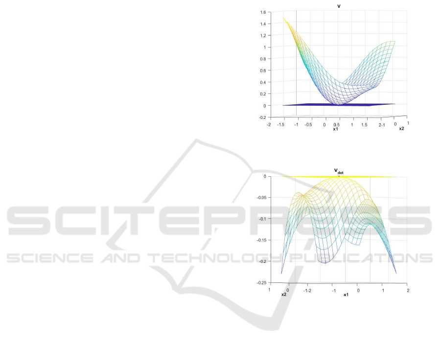
Figure 1: The constructed Lyapunov function for this sys-
tem.
Figure 2: The time derivative of the constructed Lyapunov
function.
We can easily check that the neural network is a Lya-
punov function for this system. Therefore, the origin
of the system is stable.
4.2.2 Nonlinear System Containing the Tangent
Function
Let us consider the following system:
(
˙x
1
= −tan x
1
+ x
2
2
˙x
2
= −x
2
+ x
1
The ranges for ˙x
1
and ˙x
2
are ˙x
1
∈ [−1,1] and ˙x
2
∈
[−1,1]. The stability of the origin is considered and
the figures 3 and 4 show the result. We can easily
check that the neural network is a Lyapunov function
for this system. Therefore, the origin of the system is
stable.
ICINCO 2020 - 17th International Conference on Informatics in Control, Automation and Robotics
178

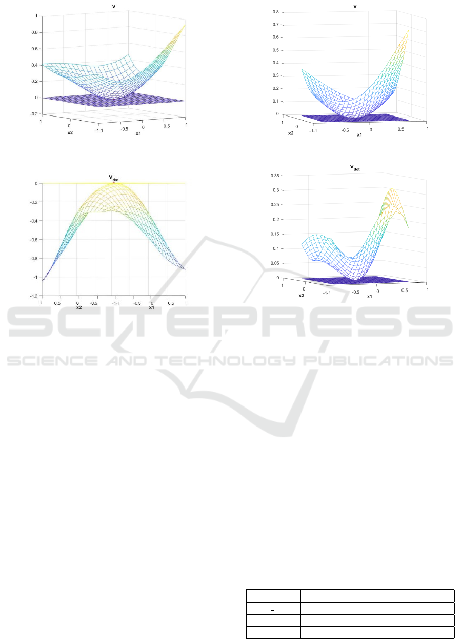
Figure 3: The constructed Lyapunov function for this sys-
tem.
Figure 4: The time derivative of the constructed Lyapunov
function.
4.3 Instability
4.3.1 Damped Pendulum
We use the same system than the first example but
instead of considering the stability of the origin, we
will consider the instability of the equilibrium point
x
e
= [π; 0].
Let us consider the following system:
(
˙x
1
= x
2
˙x
2
= −sin x
1
− x
2
The ranges for ˙x
1
and ˙x
2
are ˙x
1
∈ [π/2, −π/2] and ˙x
2
∈
[−1,1]. The instability of x
e
= [π; 0] is considered and
the figures 5 and 6 show the result:
We can easily check that the neural network is a
Chetaev function for this system. Therefore, the equi-
librium point x
e
= [π; 0] of the system is unstable.
4.4 Performance Measurement
Since the optimization algorithm tested is stochastic,
a statistical analysis of the results is required. Thus,
the performance measurement rule is as follows.
Figure 5: The constructed Chetaev function for this system.
Figure 6: The time derivative of the constructed Chetaev
function.
The cost function Q is defined in 3.2 for the sta-
bility cases and J in 3.3 for the instability case. We
are going to use only the notation Q for the two costs
functions to simplify the notation in this section. Each
test of each system is subjected to 10 successive runs:
we note the minimum value of Q obtained (Q
min
), the
mean value of Q (Q
mean
), its standard deviation (Q
std
)
and finally, the average calculation time (t
cpu
) taken to
perform these 10 runs. The results are presented in ta-
ble 1.

















Q
min
= min
i=1,...,nruns
Q
i
Q
mean
=
1
n
nruns
∑
i=1
Q
i
Q
std
=
s
1
n
n runs
∑
i=1
(Q
i
− Q
mean
)
2
(18)
Table 1: Algorithm Performance Measurement.
Q
min
Q
mean
Q
std
t
cpu/run(mn)
Stab 4.1.1 - 1 - 0.95 0.16 68.3
Stab 4.1.2 - 1 -1 0 52.6
Instability - 1 -1 0 47.5
Efficient Construction of Neural Networks Lyapunov Functions with Domain of Attraction Maximization
179

According to the definition of problems Q and J , a
neural network candidate is a Lyapunov function or
a Chetaev function if Q < 0 in the table 1. In these
cases, we have the best domain if Q = - 1.Therefore,
we see that our approach has very good results. The
optimization algorithm finds a Lyapunov function 29
times out of 30 runs with these 2 examples. The best
runs lead to the figures presented in the section Simu-
lation Results.
5 CONCLUSIONS
In this paper, we were investigating a new approach
for the construction of a Lyapunov function modelled
by a Neural network with the optimization of the do-
main of attraction. We propose to use a new con-
strained method such that the weights of the neural
network is calculated in a way that is proven mathe-
matically that the result function is a Lyapunov func-
tion while maximizing the DOA. Future works deals
with proving more complex stability properties, such
as the exponential, the robust stability and the Input-
to-state stability (ISS). Besides, future works deals
with develop this algorithm for real complex systems
that we can find in industrial framework and for dis-
crete time systems.
REFERENCES
Arg
´
aez, C., Giesl, P., and Hafstein, S. F. (2018). Iterative
construction of complete lyapunov functions. In SI-
MULTECH, pages 211–222.
Banks, C. (2002). Searching for lyapunov functions using
genetic programming. Virginia Polytech Institute, un-
published.
Chetaev, N. (1934). Un th
´
eoreme sur l’instabilit
´
e. In Dokl.
Akad. Nauk SSSR, volume 2, pages 529–534.
Feyel, P. (2017). Robust control optimization with meta-
heuristics. John Wiley & Sons.
Giesl, P. and Hafstein, S. (2015). Review on computational
methods for lyapunov functions. Discrete and Contin-
uous Dynamical Systems-Series B, 20(8):2291–2331.
Khalil, H. K. and Grizzle, J. W. (2002). Nonlinear systems,
volume 3. Prentice hall Upper Saddle River, NJ.
Krishna, A. V., Sangamreddi, C., and Ponnada, M. R.
(2019). Optimal design of roof-truss using ga in mat-
lab. i-Manager’s Journal on Structural Engineering,
8(1):39.
Long, Y. and Bayoumi, M. (1993). Feedback stabilization:
Control lyapunov functions modelled by neural net-
works. In Proceedings of 32nd IEEE Conference on
Decision and Control, pages 2812–2814. IEEE.
Lyapunov, A. M. (1892). The general problem of the sta-
bility of motion. International journal of control,
55(3):531–534.
Panikhom, S. and Sujitjorn, S. (2012). Numerical approach
to construction of lyapunov function for nonlinear sta-
bility analysis. Research Journal of Applied Sciences,
Engineering and Technology, 4(17):2915–2919.
Petridis, V. and Petridis, S. (2006). Construction of neu-
ral network based lyapunov functions. In The 2006
IEEE International Joint Conference on Neural Net-
work Proceedings, pages 5059–5065. IEEE.
Prokhorov, D. V. (1994). A lyapunov machine for stability
analysis of nonlinear systems. In Proceedings of 1994
IEEE International Conference on Neural Networks
(ICNN’94), volume 2, pages 1028–1031. IEEE.
Serpen, G. (2005). Empirical approximation for lyapunov
functions with artificial neural nets. In Proceedings.
2005 IEEE International Joint Conference on Neural
Networks, 2005., volume 2, pages 735–740. IEEE.
ICINCO 2020 - 17th International Conference on Informatics in Control, Automation and Robotics
180