
Definition of a Walking with Starting and Stopping Motions for the
Humanoid Romeo
A. Kalouguine
1,2 a
, V. de-Le
´
on-G
´
omez
1
, C. Chevallereau
1 b
, S. Dalibard
2 c
and Y. Aoustin
1,∗ d
1
Laboratoire des Sciences du Num
´
erique de Nantes, CNRS UMR 6004, Ecole Centrale de Nantes,
Universit
´
e de Nantes, France
2
SoftBank Robotics, 43, Rue du Colonel Pierre Avia, 75015, Paris, France
Keywords:
Humanoid Robot, Starting Motion, Stopping Motion, Center of Mass, Zero Moment Point, Essential Model.
Abstract:
The aim of this paper is to develop a complete walking with a starting, periodic and stopping motion for a 3D
humanoid robot with n actuated variables. The dynamic behaviour of the center of mass of the humanoid robot
is defined by a model called Essential model. The ZMP is imposed, the horizontal position of the CoM is free.
The n − 2 other generalized variables of the humanoid robot are controlled and their trajectories can be for
example chosen as a sinusoidal function of time. The gait parameters are determined based on data obtained
from human walking. Numerical tests are presented for a complete walking motion. The perspectives are to
test the obtained trajectories experimentally.
1 INTRODUCTION
Designing a walking trajectory for a humanoid robot
entails strong difficulties such as unilateral constraints
with the ground, numerous joints, respecting the dy-
namic equilibrium, among others. There exist several
popular methods, which are based on the relation be-
tween the zero moment point (ZMP) and the center of
mass (CoM), to develop walking trajectories for ex-
periments with humanoid robots, for example (Kajita
et al., 2014), (Kaneko et al., 2004). Their main ad-
vantage is to not require a lot of information about
the dynamic behavior of each of the robot’s bodies.
However during a walking, an important flexion of
the knee joint for the stance leg is actually not human-
like. Also, the results are based on a simplified model,
thus the walking stability is not ensured for a robot
with small feet. With the linear inverted pendulum
(LIP) model, walking motions based on capture point
regulation are developed in order to exploit the nat-
ural dynamic of the pendulum to stop it. The cap-
ture point is the location on the ground where a biped
needs to step in order to come to a stop. The CoM
motion freely converges to the capture point, see (En-
a
https://orcid.org/0000-0003-3092-9534
b
https://orcid.org/0000-0002-1929-5211
c
https://orcid.org/0000-0001-8655-8619
d
https://orcid.org/0000-0002-3484-117X
∗
Corresponding author
glsberger et al., 2001) and (Pratt et al., 2012). But
its theoretical concept is mainly based on the assump-
tion that the altitude of the CoM is constant, i.e. the
linear inverted pendulum (LIP) assumption. A walk-
ing gait based on human-like virtual constraints has
been investigated in (Ames et al., 2012) for the robot
Nao; Sakka in (Sakka, 2017) also performed this type
of study for an online human motion imitation with
Nao for slow motions. Another approach employed
to generate walking patterns for biped robots is based
on central pattern generators (CPGs) and does not re-
quire any physical model of the biped; see (Behnke,
2006), (Graf et al., 2009) or (Shachykov, 2019). How-
ever they request the tuning of a lot of parameters.
The parametric optimisation can also be used to de-
fine offline walking trajectories for humanoid robots,
for example (Bessonnet et al., 2002), (Tlalolini et al.,
2010), or (Ames et al., 2012). The main advantage
of parametric optimization is that energy consump-
tion can be minimized. But this method requests a lot
of computation efforts. The reference motion of the
biped can also be based on a record of human mo-
tion (Powell et al., 2013), (Tomic et al., 2014). By
definition, a human is a perfect model to define a hu-
manoid walking. Nevertheless, making the correla-
tion between the human motion and the robot joints
is not so easy. Despite these interesting contributions,
to our best knowledge there are few papers about the
design of a complete walking motion, taking into ac-
Kalouguine, A., de-León-Gómez, V., Chevallereau, C., Dalibard, S. and Aoustin, Y.
Definition of a Walking with Starting and Stopping Motions for the Humanoid Romeo.
DOI: 10.5220/0009827000470055
In Proceedings of the 17th International Conference on Informatics in Control, Automation and Robotics (ICINCO 2020), pages 47-55
ISBN: 978-989-758-442-8
Copyright
c
2020 by SCITEPRESS – Science and Technology Publications, Lda. All rights reserved
47
count the constraints on ZMP trajectory, with a start-
ing, a periodic and a stopping motion. An interest-
ing investigation was done in (Ames, 2014) but the
approach was more hybrid, without double support
phases. In (Khusainov et al., 2017), desired foot po-
sitions of the humanoid robot are generated for any
given trajectory by taking into account kinematic lim-
its in robot legs. In but to our best knowledge for hu-
manoid robots there are no extract trajectories from
human data.
The contribution of this paper is to fill this gap.
Our main objective is to find feasible walking trajec-
tories for a given robot, taking into account these dy-
namic characteristic, i.e. with unilateral ground con-
tact forces and ensure dynamic equilibrium. More-
over, the proposed trajectories are inspired by aver-
age human motion, copying a particular human gait,
chosen to translate an emotion like joy or fatigue, or
dedicated to a task like carrying loads, etc. A com-
plete walking motion is defined for Romeo, a hu-
manoid robot with n = 31 joints. This complete walk-
ing, which is composed of double support (DS) and
single support (SS) phases is calculated by using the
Essential model, which models the relation between
ZMP and CoM by considering the complete dynamic
of the robot unlike the LIP model, i.e. a determin-
ing feature of human gait, (De-Le
´
on-G
´
omez et al.,
2019). Vukobratovic (Vukobratovic et al., 2012) en-
lighten us on biomechanical inspiration of this feature
to carry out biped robot motion such as posture real-
ization, gait synthesis. The trajectory of the ZMP is
here imposed, the horizontal position of the CoM of
the humanoid robot is free to adapt to the ZMP evolu-
tion. The n−2 remaining generalized coordinates are
given functions of time (often sinusoidal functions),
whose parameters are inspired by data extracted from
human walking. The CoM is thus computed from
the knowledge of the evolution of the ZMP and these
n − 2 remaining generalized coordinates. The n joint
variables of the robot are deduced from this calcula-
tion. From the inverse dynamic model it is possible to
deduce the torques to carry out this complete walking.
The paper is outlined as follows. The humanoid
robot Romeo is described in section 2. The Essential
model is presented in section 3. The boundary value
problem to obtain a periodic walking motion is stated
in section 4. The starting and stopping phases are de-
tailed in section 5. The results of the numerical tests
are presented in section 6. Section 7 offers our con-
clusions and perspectives.
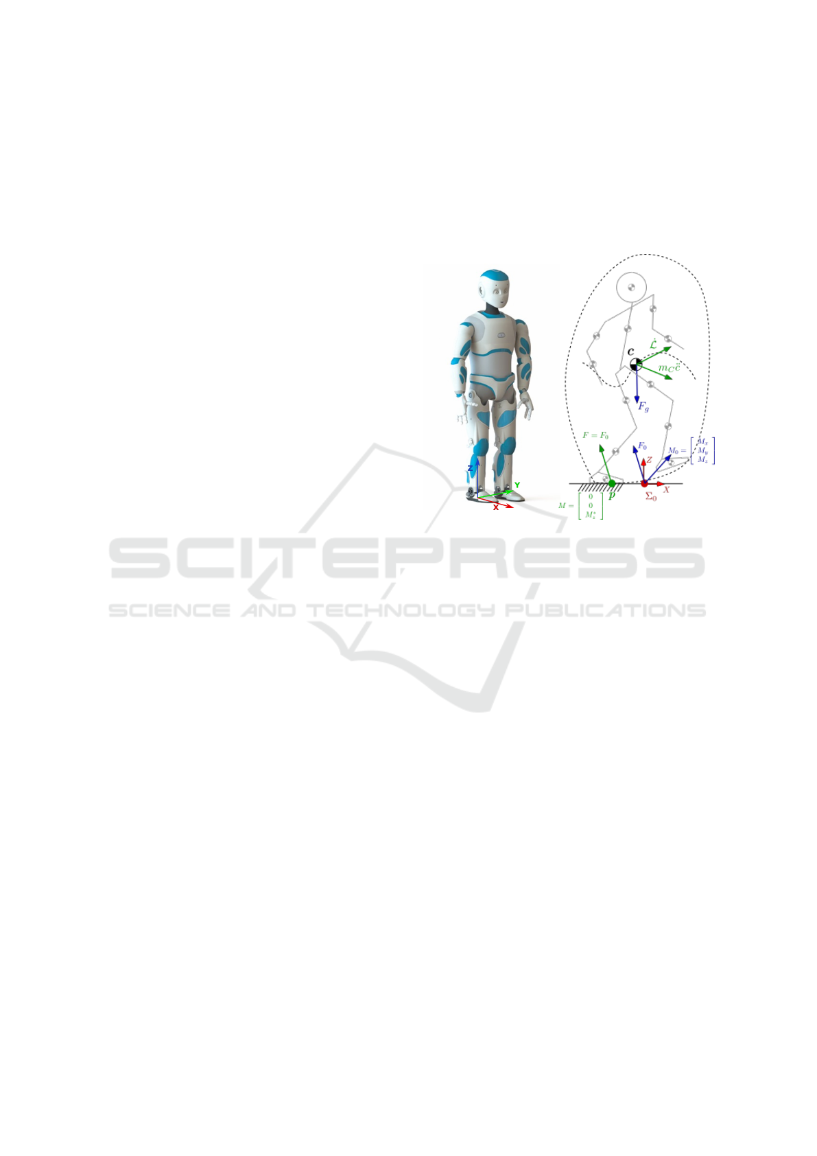
2 ROMEO
The humanoid robot considered in this study is
Romeo, a prototype platform developed by the com-
pany Softbank Robotics, see fig. 1 a). It is 1.47m
tall, weighs 36 kg and features 31 degrees of freedom
(DoF) gathered into the configuration vector q.
a)
b)
Figure 1: A) Photography of Romeo. b) Illustration of the
global equilibrium.
3 ESSENTIAL MODEL
The objective of the Essential model is, instead of im-
posing as many trajectories as there are degrees of
freedom (DoFs), to leave two DoFs free to allow for a
chosen placement of the ZMP. Since the relation be-
tween ZMP and CoM is considered as a determining
feature of human gait (Kajita et al., 2014), (Koolen
et al., 2012), and the positions of CoM and ZMP are
strongly linked, we choose to ”set free” the horizontal
coordinates r
f
= (x, y) of the CoM in order to adapt
to the imposed trajectory of the ZMP.
In order to take inspiration from the human motion,
let us introduce r ∈ R
31×1
:
r = (r
f
, r
c
)
>
= (x,y, z(t), x
f
(t), y
f
(t), z
f
(t), ψ
f
(t), θ
f
(t),
φ
f
(t), ψ
t
(t), θ
t
(t), φ
t
(t), q
13
(t), ·· · , q
31
(t))
>
.
(1)
We define r
c
as the vector of the 29 variables of r
for which the trajectories are imposed. z(t) defines
the desired altitude of the CoM. x
f
(t), y
f
(t), z
f
(t) and
ψ
f
(t), θ
f
(t), φ
f
(t) describe the desired position and
orientation of the free foot, and ψ
t
, θ
t
, φ
t
give the de-
sired orientation of the torso link. The upper-body
ICINCO 2020 - 17th International Conference on Informatics in Control, Automation and Robotics
48

variable joints are defined by q
13
to q
31
. The desired
trajectory for r
c
(t) is defined based on human motion.
The robot configuration can be defined by the joint
vector q ∈ R
31×1
or by the vector r, and a geometric
model can be built. Let q = g(r
f
, r
c
) be, ˙q and ¨q are
deduced thanks to the kinematic models as follows:
˙q = J
f
˙r
f
+J
c
˙r
c
, ¨q = J
f
¨r
f
+
˙
J
f
˙r
2
f
+J
c
¨r
c
+
˙
J
c
˙r
2
c
. (2)
Here J
f
∈ R
31×2
and J
c
∈ R
31×29
. In this study the
evolution of r
c
is chosen as a function of time, thus
the joint evolution can be expressed as function of
r
f
, ˙r
f
, ¨r
f
and t only :
q = g(r
f
,t), ˙q = J
f
˙r
f
+ v(t, r
f
),
¨q = J
f
¨r
f
+
˙
J
f
˙r
2
f
+ a(t, r
f
, ˙r
f
).
(3)
To assess the feasibility of a walking trajectory,
it is necessary to calculate the external forces act-
ing on the humanoid robot. These external forces
here are the gravity force F
g
and the ground reac-
tion forces applied on each foot (see fig. 1 b). The
resulting ground reaction is defined by the wrench ∈
R
6×1
(F
0
, M
0
)
>
= (F
x
, F
y
, F
z
, M
x
, M
y
, M
z
)
>
in a refer-
ence frame Σ
0
. The global equilibrium of the robot
can be written as :
F
0
M
0
=
A
F
A
M
¨q +
d
F
(q, ˙q)
d
M
(q, ˙q)
(4)
where q ∈ R
31×1
is the joint vector of the robot.
Using (3), the global equilibrium (4) can be
rewritten:
F
0
M
0
=
A
Fr
(t, r
f
)
A
Mr
(t, r
f
)
¨r
f
+
d
Fr
(t, r
f
, ˙r
f
)
d
Mr
(t, r
f
, ˙r
f
)
(5)
Let p = (p
x
, p
y
, 0)
>
be the global zero moment point
(ZMP). Its coordinates p
x
and p
y
satisfy :
F
z
p
x
+ M
y
= 0, F
z
p
y
− M
x
= 0.
(6)
(p
x
, p
y
) must be inside the convex hull of support at
all times in order to satisfy the dynamic equilibrium
condition (Vukobratovic and Borovac, 2004). We im-
pose a desired evolution of the ZMP px(t) and py(t)
inside the convex hull of the support foot (or feet in
DS) in order to satisfy the equilibrium condition. Dur-
ing the SS phase the desired motion of the ZMP is a
migration of the ZMP from the heel to the toe of the
stance foot. In DS phase the desired motion of the
ZMP is defined by a linear evolution from the final
position of the ZMP at the end of the SS phase on the
stance foot, until the initial position of the ZMP at the
beginning of the SS on the next stance foot. By using
the 3
th
, 4
th
, and 5
th
lines of (5), we rewrite (6) as:
(A
Frz
(t, r
f
)¨r
f
+ d
Frz
(t, r
f
, ˙r
f
)) p
x
(t)+
A
Mry
(t, r
f
)¨r
f
+ d
Mry
(t, r
f
, ˙r
f
) = 0,
(A
Frz
(t, r
f
)¨r
f
+ d
Frz
(t, r
f
, ˙r
f
)) p
x
(t)−
A
Mrx
(t, r
f
)¨r
f
− d
Mrx
(t, r
f
, ˙r
f
) = 0.
(7)
These two scalar equations (7) isolate the essential
characteristic of the walking that is the relationship
between the ZMP and the CoM. Solving (7) gives
the Essential model describing the acceleration of the
horizontal positions x and y of the CoM, that are de-
fined to achieve the imposed evolution of the ZMP:
¨r
f
= f (r
f
, ˙r
f
,t, p
x
(t), p
y
(t)). (8)
By integration of (8) from initial conditions we
can calculate the current values of ˙r
f
, i.e. ˙x, ˙y, and
r
f
, i.e x, and y. To sum up, the evolution of x and y is
not imposed in order to allow them to adapt to the im-
posed evolution of the ZMP. With this strategy to de-
fine a reference trajectory of walking, which is based
on the Essential model (8) and r
c
(t), no approxima-
tions are made to the dynamic model when designing
the humanoid walking. The method ensures the fea-
sibility of a walking trajectory from the point of view
of the condition on the ZMP.
The choice of the height z(t) of the CoM allows to
satisfy the positivity of the vertical component of the
resultant ground reaction force during the walking. It
is sufficient to satisfy
¨z(t) > −g
The condition of no slipping can be checked based on
the knowledge of ¨r
f
and ¨z. It is sufficient to satisfy
||¨r
f
(t)|| < µ(¨z(t) − g)
where µ is the friction coefficient. The numerical val-
idation of these conditions is presented in fig. 9.
3.1 Torques and Ground Forces in SS
and DS
By now, the torques required to produce the motion
have to be calculated. During the SS phase, by con-
sidering the stance foot motionless on the ground, we
can define the dynamic behavior of the robot:
τ = A
r
(t, r
.
f )¨r
f
+ d
r
(t, r
f
, ˙r
f
) (9)
In DS phase, the effort wrench (F
ext
, M
ext
)
>
applied
on the second leg, (9) becomes
τ = A
r
(t, r
f
)¨r
f
+ d
r
(t, r
f
, ˙r
f
) + J
ext
F
ext
M
ext
. (10)
The global equation gives the global reaction effort
F
0
, M
0
, but the distribution on both legs is free and
will modify the actuation torque. During a DS, the
global ZMP is the barycentre of the two local ZMPs
on each foot, this implies that the global ZMP and the
local ZMPs are aligned. In DS, the choice of local
ZMPs p
1
and p
2
is used to calculate the distribution
Definition of a Walking with Starting and Stopping Motions for the Humanoid Romeo
49

of efforts. This choice must limit the internal forces
useless to the motion in order to avoid increasing the
joint torques. We can then calculate the vertical reac-
tion force F
1z
and F
2z
on legs 1 and 2 by solving this
system:
p
1x
F
1z
+ p
2x
F
2z
F
1z
+ F
2z
= p
x
p
1y
F
1z
+ p
2y
F
2z
F
1z
+ F
2z
= p
y
(11)
To limit the risk of slipping, the ratio between tangen-
tial and normal forces for the global equilibrium is
chosen equal for each leg. The components F
1x
, F
1y
,
F
2x
, and F
2y
are calculated to satisfy:
F
1x
F
1z
=
F
2x
F
2z
=
F
1x
+ F
2x
F
1z
+ F
2z
F
1y
F
1z
=
F
2y
F
2z
=
F
1y
+ F
2y
F
1z
+ F
2z
(12)
By using (11) and (12) we find M
z
= M
1z
+ M
2z
. The
moment around the z axis is also shared between the
two legs by using a similar distribution to the force
components (12) as follows:
M
1z
F
1z
=
M
2z
F
2z
=
M
1z
+ M
2z
F
1z
+ F
2z
(13)
In this study, two types of DS phases are consid-
ered.
• DS during the walking phase which allows to join
two phases of SS with foot positions offsets along
the x and y axes. We want to have a continuous
evolution of the ZMP, which results in continuous
joint torques and avoids high jerk. We choose an
evolution of the global ZMP in order that during
the DS phases, the two local ZMPs keep a con-
stant pose corresponding to the final pose of the
ZMP in SS: p
1
, and the initial pose of the ZMP
for the next SS: p
2
. This implies that the global
ZMP evolves linearly between the final pose of
the ZMP during the previous SS and the initial
pose of the ZMP during the next SS.
• For the initial DS in starting phase, or the final DS
in stopping phase, on the contrary, we have the
two feet aligned along the x-axis and a non-linear
evolution of the global ZMP (Jian et al., 1993).
The local ZMPs will then be chosen to yield the
current value of the global ZMP along the x-axis
while remaining within the surface of the corre-
sponding foot. In addition, when stationary, we
want an identical distribution of forces over the
two feet, we choose a position of the CoM accord-
ing to the y-direction between the two feet and a
y-position of the local ZMPs in the center of the
feet. A linear ZMP evolution along the y-axis is
chosen. The aim is to ensure continuity and to
minimize the lateral torque on the ankle. An illus-
tration is shown in fig. 8 for the case studied.
4 PERIODIC WALKING MOTION
The periodic motion is composed of SS phases and
DS phases with flat foot contacts on the ground. There
is no impact at the end of the SS phase, since the ve-
locity of the swing foot is imposed to be zero when
it touches the ground. A quadratic-cycloidal function
is used to define the trajectory of the swing foot. The
orientation of its sole is varying during motion, but
parallel to the ground during DS phases. Sinusoidal
functions are used to define the motions of the arms
and the trunk. The parameters of these functions are
tuned based on observations of human motions (Win-
ter, 1992). To define a periodic walking motion for
Romeo, the step width D and the step length S are
adapted to its physical characteristics and the limits of
its actuators. The step width D is chosen to be 0.20m
to satisfy a safe clearance between Romeo’s ankles.
The step length S is chosen in the range 0.15 to 0.20m,
which corresponds to a 0.30-0.40m displacement of
the swing foot and a velocity of 0.83 to 1.1km/h re-
spectively. The duration of one DS phase is chosen to
be close to 12% of the cycle (2 steps) duration 2 · T ,
where T = T
DS
+T
SS
. T
DS
= 0.15s and T
SS
= 0.60s are
the chosen durations of the DS phases and SS phases.
In SS, the ZMP evolution is chosen as linear along the
x axis and centered in the middle of the foot along the
y axis. In DS, the ZMP evolves linearly between its
final position in the previous SS and its initial position
in the next SS as explained in section 3.1.
To find the periodic motion, a boundary value
problem is stated and solved as follows. Let
(x(t
0
), y(t
0
), ˙x(t
0
), ˙y(t
0
)) be the components in the hor-
izontal plane of the position and velocity of the COM
at the beginning of a current step of the walking mo-
tion. The periodic condition is
(x(t
0
), y(t
0
), ˙x(t
0
), ˙y(t
0
)) =
(x(t
0
+ T ), y(t
0
+ T ), ˙x
+
(t
0
+ T ), ˙y
+
(t
0
+ T ))
(14)
by taking into account the change of the reference
frame when the two legs switch their roles just at the
beginning of the current step. So ˙x
+
(t
0
+ T ), ˙y
+
(t
0
+
T ) are the initial velocities of the COM in SS of the
next step. The boundary value problem is stated as:
what are x(t
0
), y(t
0
), ˙x(t
0
) and ˙y(t
0
) such that after in-
tegration of (8) over the time interval [t
0
,t
0
+ T ] the
periodic condition (14) is satisfied.
ICINCO 2020 - 17th International Conference on Informatics in Control, Automation and Robotics
50

5 STARTING AND STOPPING
MOTIONS
In order to perform the target periodic walking mo-
tion experimentally, it is necessary to add starting and
stopping motions, which are composed of DS phases
and SS phases. This allows the robot to start from
(resp. to stop in) a resting position. Each resting posi-
tion is defined to be a static equilibrium where the ver-
tical projection of the CoM on the ground is merged
with the ZMP close to the center of the convex hull
of support. From the observation of data from human
walking (Grundy et al., 1975) a ZMP trajectory is de-
fined by using piecewise polynomial functions to be
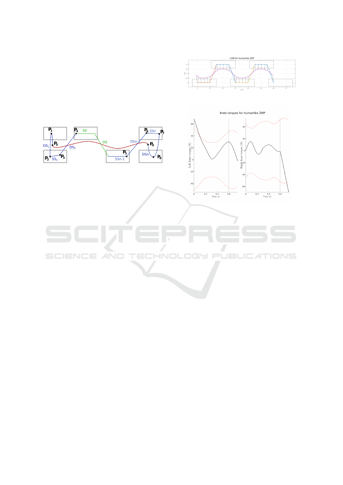
adapted to a humanoid robot. A sequence of starting
phase (DS
1
, SS
1
, and DS
2
), a periodic walking motion
(SS and DS) and a stopping phase (SS
n−1
, DS
n−1
, SS
n
,
and DSS
n
) is shown in fig. 2.
For the starting motion control points are intro-
duced:
• P
0
ZMP at the start of DS
1
• P
1
ZMP in the middle of DS
1
• P
2
ZMP at the transition between DS
1
and SS
1
• P
3
ZMP at the transition between SS
1
and DS
2
• P
4
ZMP at the end of the DS
2
phase
These control points are used to define the evolution
of ZMP during starting phase. They are illustrated on
fig. 2
In DS
1
phase p
x
and p
y
are both defined as
quadratic functions of time going from P
0
to P
2
with
the intermediate point P
1
. In SS
1
and DS
2
phases p
x
and p
y
are defined as linear functions of time con-
necting, respectiively, P
2
to P
3
and P
3
to P
4
. P
4
is
imposed by the chosen periodic trajectory.
For the stopping motion, the strategy to define the
ZMP trajectory is similar. We define:
• P
5
ZMP at the transition between SS
n−1
and
DS
n−1
• P
6
ZMP at the transition between DS
n−1
and SS
n
• P
7
ZMP at the transition between SS
n
and DS
n
• P
8
ZMP in the middle of DS
n
• P
9
ZMP at the end of the DS
n
phase
At the start of SS
n−1
phase, the ZMP position is
(taking into account the change of reference frame)
the same as in P
4
because of the periodic nature of
the trajectory before SS
n−1
. We can therefore denote
this point as P
4
as well. In SS
n−1
phase, p
x
and p
y
are
therefore defined as linear functions to connect P
4
to
P
5
. In DS
n−1
and SS
n
phases, p
x
and p
y
are defined as
linear functions of time to connect P
5
to P
6
, P
6
to P
7
,
respectively. In DS
n
phase p
x
and p
y
are defined as
quadratic functions of time connecting P
7
to P
9
with
an intermediate point P
8
.
The stopping phase with two DS phases and two
SS phases is not symmetric with respect to the start-
ing phase with two DS phases and only one SS phase
in order to mimic easier the motion of the ZMP in hu-
mans during the starting and stopping motions. The
step width D and the step length S are given but
not necessarily similar between the starting, stopping
and periodic motions. A boundary value problem is
solved to define the starting and stopping motions.
This boundary value problem is stated as follows:
Starting Motion. Let us consider the known two co-
ordinates of the horizontal position of the CoM,
which is also the ZMP position P
0
. Their two
velocities are equal to zero. Let us consider the
known two coordinates of the horizontal position
of the CoM at the end of DS
2
phase and their two
velocities. These two coordinates and two veloc-
ities are also the state of the periodic horizontal
motion of the CoM at the beginning of the SS
phase.
Let us take into account the essential model
(8) and T
start
the duration of the starting mo-
tion. What are the four possible variables
to carry out the starting motion by integra-
tion of (8) from (X(0),Y (0),
˙
X(0),
˙
Y (0))
>
to
(X(T
start
),Y (T
start
),
˙
X(T
start
),
˙
Y (T
start
))
>
? We
choose the components p
x
and p
y
of the two con-
trol points P
2
, and P
3
of the ZMP trajectory, to
solve this boundary problem. A SQP method (Se-
quential Quadratic Programming) with fmincon of
Matlab
R
is used to find the coordinates of P
2
,
and P
3
in order to easier ensure that the ZMP is
always inside of the convex hull of the support
area. The Essential model dynamics are then in-
tegrated from the starting state (r
f
(0), ˙r
f
(0))
>
for
this COM, to the final state (r
f
(T
start
), ˙r
f
(T
start
))
>
of the starting motion. This final state is compared
to the target state (r
des
f
(T
start
), ˙r
des
f
(T
start
))
>
by us-
ing a Mean Square criterion (optionally weighed
to emphasize the importance of one of the dimen-
sions):
J = (X(T
start
) − X
des
(T
start
))
2
+
(Y (T
start
) −Y
des
(T
start
))
2
+
(
˙
X(T
start
) −
˙
X
des
(T
start
))
2
+
(
˙
Y (T
start
) −
˙
Y
des
(T
start
))
2
.
(15)
Stopping Motion. The strategy is similar to that of
the starting motion. For the four possible vari-
ables to carry out the stopping motion we choose
Definition of a Walking with Starting and Stopping Motions for the Humanoid Romeo
51
the components p
x
and p
y
of the two control
points P
6
to P
7
of the ZMP trajectory, to solve this
boundary problem. An equivalent criterion to (5)
is calculated with respect to the two coordinates
of the horizontal resting position of the CoM and
their two respective velocities.
J = (X(T
stop
) − X
des
(T
stop
))
2
+
(Y (T
stop
) −Y
des
(T
stop
))
2
+
˙
X(T
stop
)
2
+
˙
Y (T
stop
)
2
.
(16)
Figure 2: Sequence starting motion, cycling walking stop-
ping motion.
All joint trajectories also need to be continuous
during this transition. And since there is no impact
in our gait, this is equivalent to imposing that the
evolution of r
c
be continuous. The sinusoidal func-
tions, which define the actuated joints of the arms and
trunk, are multiplied by a piecewise polynomial cut-
off function which is equal to 1 during the periodic
motion and smoothly goes to 0 during the starting and
stopping phases in order to start and to stop with a null
velocity and null acceleration.
6 NUMERICAL RESULTS
6.1 Periodic Motion
We choose a ZMP trajectory close to the one that is
observed in humans. Since we do not have foot roll-
off motion, we avoid the ZMP reaching the edges of
the foot. That way, the non-tilting condition is safely
satisfied.
The evolution of ZMP in DS phase is chosen as
follows:
• In x-direction, from p
x
= 0 (under the ankle) to
p
x
= 0.10m (in the toes of the foot).
• In y-direction, p
y
= 0 (center of the foot).
The corresponding COM trajectory is represented
on fig. 3. We observe that the COM trajectory in
the horizontal plane is not far from a sinus func-
tion, which is what is observed for humans (Rose and
Gamble, 2006).
However, when calculating the torque values for
this trajectory, we observe that the torques are not
Figure 3: COM trajectory corresponding to a human-like
evolution of the ZMP.
Figure 4: Torques at both knees for a human-like ZMP tra-
jectory. The dashed line marks the end of the SS phase
(swing foot contact), and the red dashed lines show the max-
imum acceptable torque for Romeo. It is interesting to note
that these limits are not constant - this is because of a speci-
ficity of the knee joint in Romeo: the maximum torque de-
pends on the joint position.
compatible with the hardware of Romeo, as shown
in fig. 4. In order to reduce these torques, we need
to make some adaptations to the original parameters.
We analyzed the effect of various parameters on the
torques, and observed that the most efficient way to
influence the knee torques is to modify the ZMP tra-
jectory. The result of this adaptation is presented in
the following section, and the trajectory used in the
rest of the paper is the modified one.
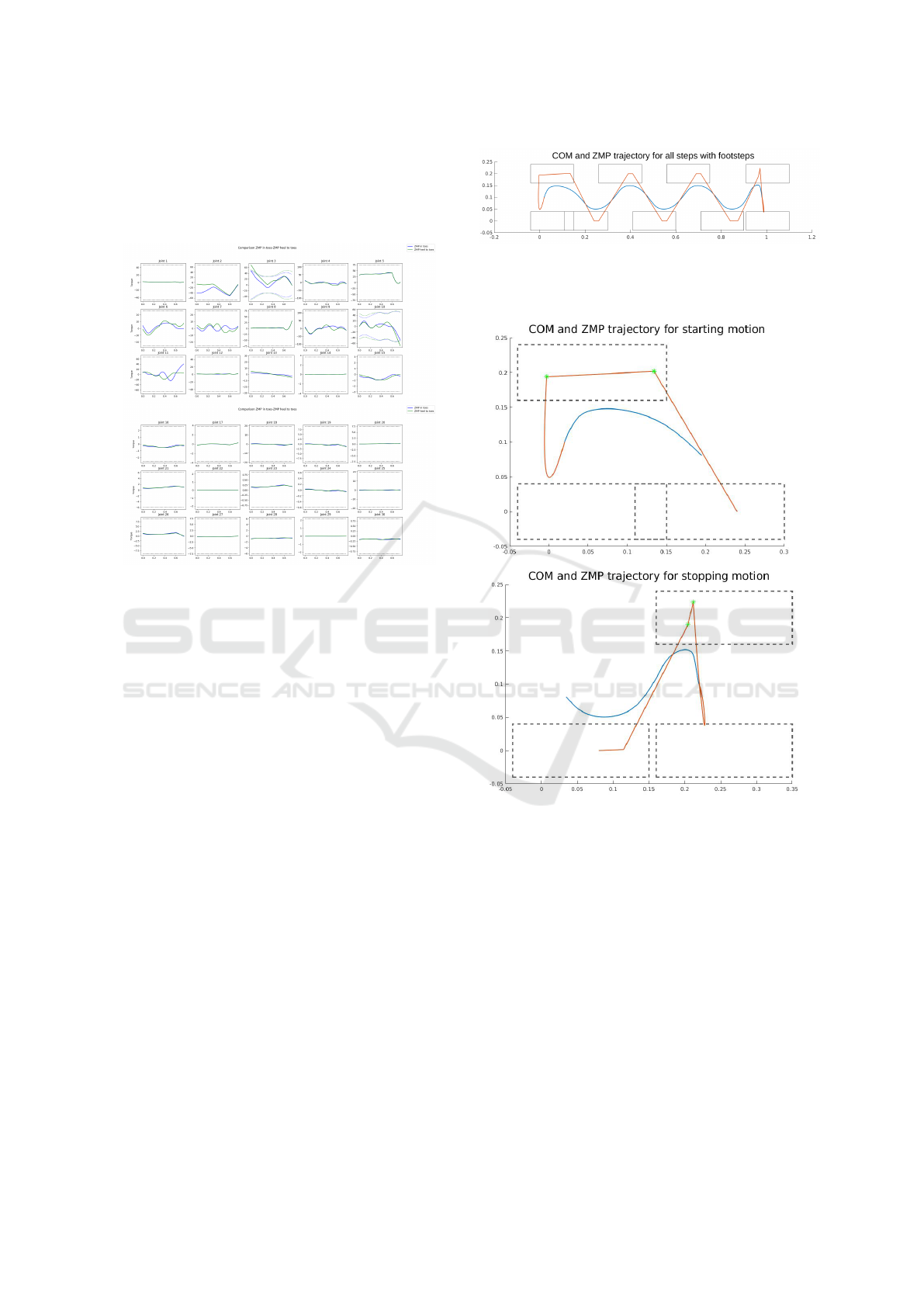
6.2 Effect of ZMP Evolution on Torques
The results presented above correspond to an evolu-
tion of the ZMP going from the heel to the tip of each
foot (see fig. 3). The torque at the ankle is directly
affected by the pose of the ZMP. It can be seen in fig.
5 (2
nd
image), that the propulsive torque at the ankle
is low at the beginning of the step. As a consequence,
a high propulsive torque is required at the knee joint
(fig. 5 (3
th
image)). In fact this high torque exceeds
the limits of the actuator (shown in dotted line) of the
robot Romeo. We explored the effect of the influence
of ZMP evolution. The results show that a modifica-
tion of the ZMP trajectory influences the torques in
the support knee and in the support ankle. A ZMP
ICINCO 2020 - 17th International Conference on Informatics in Control, Automation and Robotics
52
that has a constant position in front of the foot allows
a higher propulsive force in the ankle at the beginning
of the SS, and thus allows to decrease the propulsive
force at knee, and then produces a knee torque com-
patible with the actuator of Romeo.
Figure 5: Joint torques (N.m) versus time (s): comparison
of the torque in the lower part of the robot for two periodic
trajectories with a step size of 0.20 m and a period of 0.75 s.
The trajectory in green is with a human like ZMP evolution
in DS, and the trajectory in blue has a ZMP constrained to
the front of the foot.
6.3 Complete Motion
The synthesised walking trajectory is such that the
step width parameter D is the same for the starting,
periodic and stopping motions. The step length pa-
rameter S is chosen to be 0.16m, 0.15m and 0.20m
for the starting, periodic and stopping motions respec-
tively. For this synthesised trajectory, the trajectories
of the horizontal position of the CoM and the ZMP
are shown fig. 6. The starting motion and the stop-
ping phases are respectively composed of three and
four phases. Four steps make up the periodic mo-
tions. During this periodic motion the step size equals
0.15m. We can observe that the COM and ZMP evo-
lutions are continuous from the starting configuration
to the stopping configuration.
A focus of the starting and stopping phases is pre-
sented fig. 7. The horizontal position of the CoM and
the ZMP position coincide well at the starting and
stopping configurations. The control points to solve
the two boundary value problems are depicted with
green stars.
In the first and last DS phases, the ZMP follows
a more complex trajectory. It is therefore necessary
Figure 6: Imposed ZMP trajectory (orange) and corre-
sponding COM (blue). The dashed rectangles represent the
foot placements.
Figure 7: Imposed ZMP trajectory (orange) and horizontal
position of the corresponding COM (blue).
to define a non constant local ZMP for each foot. We
choose at all times to keep the same x coordinate as
the global ZMP, and stay as close as possible to the
center of each foot in y direction to improve walking
stability. The resulting local ZMP trajectories are pre-
sented in fig. 8.
We can also verify that the non slipping condition
is fulfilled. This condition is the fact that the ratio be-
tween the tangential and normal forces does not ex-
ceed the friction coefficient. This friction coefficient
is chosen equal to 0.7 here. Both of these forces are
calculated with (4). The sinusoidal-like shape of the
normal reaction force observed in fig. 9 is linked to
the oscillations of the height z the COM F = m¨z +mg.
Definition of a Walking with Starting and Stopping Motions for the Humanoid Romeo
53
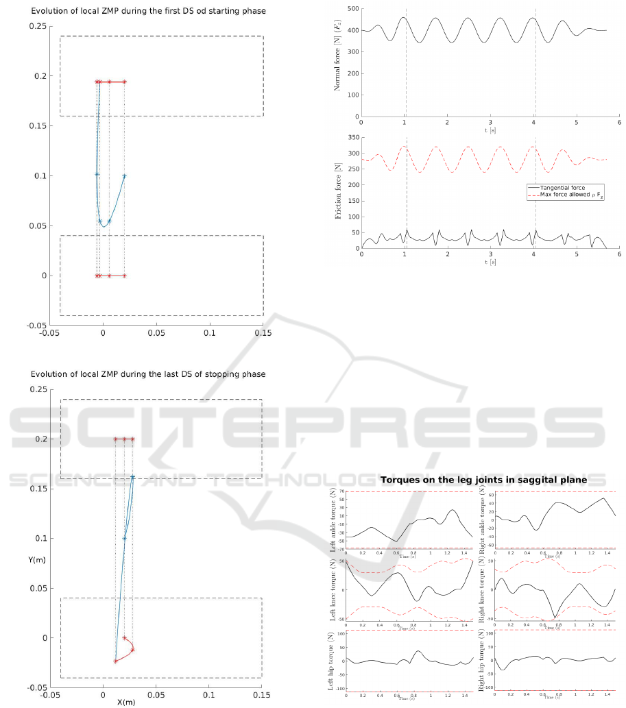
a)
b)
Figure 8: Evolution of the local ZMP (red) for each foot
respectively during the first and last DS phases of the start-
ing (a) and stopping (b) motions. The blue line indicates
the corresponding COM evolution, resp. starting and stop-
ping in the middle of both feet. The dashed lines show the
distribution of the global ZMP and its relation to the COM
position.
Figure 9: Normal (top plot) and tangential (bottom) com-
ponents of the reaction force. The red dashed line repre-
sents the maximum acceptable tangential force without risk
of slipping.
We compute the torque value for all of the joints.
However, we choose to only present in fig. 10 the
torques on both legs in the joints in the sagittal plane.
Indeed, these are the torques that require the highest
magnitude. It can be observed that the torques are in-
side to motor limits for the studied robot. The torque
required for starting, periodic, and stopping motions
are of similar magnitude.
Figure 10: The torque at the ankle, knee and hip joints, in
the sagittal plane for the complete motion.
7 CONCLUSIONS
A complete walking with a starting motion and a stop-
ping motion is defined thanks to a strategy based on
the Essential model. This methodology ensures the
ICINCO 2020 - 17th International Conference on Informatics in Control, Automation and Robotics
54

feasibility of the walking trajectory with respect to
the condition on the ground reaction force: take off,
slipping and rotation of the support foot are avoided.
The ZMP trajectory is ensured to be inside a convex
hull of the support surface. The parameters of trajec-
tories of the swing leg ankle, the trunk and the arms
are tuned thanks to observations from human walking.
The effect of the choice of the ZMP evolution on the
required torque is investigated. A correlation between
the pose of the ZMP in sagittal plane and torque at an-
kle and knee in saggital plane has been shown. The
perspectives are to test this complete walking motion
experimentally.
REFERENCES
Ames, A. D. (2014). Human-inspired control of bipedal
walking robots. IEEE Transactions on Automatic
Control, 59(5):1115–1130.
Ames, A. D., Cousineau, E. A., and Powell, M. J. (2012).
Dynamically stable bipedal robotic walking with nao
via human-inspired hybrid zero dynamics. In Proc. of
the 15th ACM int. conf. on Hybrid Systems: Compu-
tation and Control, pages 135–144. ACM.
Behnke, S. (2006). Online trajectory generation for om-
nidirectional biped walking. In Proc. Int. Conf.
on Robotics and Automation (ICRA), pages 1597–
1603, Orlando, USA.
Bessonnet, G., Chesse, S., and Sardin, P. (2002). Generating
optimal gait of a human-sized biped robot. In Proc. of
the fifth Int. Conf. on Climbing and Walking Robots,
pages 717–724.
De-Le
´
on-G
´
omez, V., Luo, Q., Kalouguine, A., P
´
amanes,
J. A., Aoustin, Y., and Chevallereau, C. (2019). An es-
sential model for generating walking motions for hu-
manoid robots. Robotics and Autonomous Systems,
112:229–243.
Englsberger, J., Ott, C., Roa, M. A., Albu-Sh
¨
affer, A., and
Hirzinger, G. (2001). Bipedal walking control based
on capture point dynamics. In Proc. Int. Conf. on
Intelligent Robots and Systems (IROS), pages 4420–
4427, San Francsico, USA.
Graf, C., H
¨
aryl, A., R
¨
ofer, T., and Laue, T. (2009). A ro-
bust closed-loop gait for the standard platform league
humanoid. In Proc. Workshop on Humanoid Soc-
cer Robots of the IEEE-RAS Int. Conf. on Humanoid
Robots, pages 30–37, Paris, France.
Grundy, M., Tosh, P., McLeish, R., and Smidt, L. (1975).
An investigation of the centres of pressure under the
foot while walking. J. of bone and joint surgery.
British volume, 57(1):98–103.
Jian, Y., Winter, D. A., Ishac, M. G., and Gilchrist, L.
(1993). Trajectory of the body cog and cop during
initiation and termination of gait. Gait & Posture,
1(1):9–22.
Kajita, S., Hirukawa, H., Harada, K., and Yokoi, K.
(2014). Introduction to humanoid robotics, volume
101. Springer.
Kaneko, K., Kanehiro, F., Kajita, S., Hirukawa, H.,
Kawasaki, T., Hirata, M., K.Akachi, and Isozumi, T.
(2004). Humanoid robot hrp-2. In Proc. IEEE Int.
Conf. on Robotics and Automation ICRA, pages 1083–
1090, New-Orleans, Louisiana, USA.
Khusainov, R., Sagitov, A., Klimchik, A., and Magid, E.
(2017). Arbitrary trajectory foot planner for bipedal
walking. In ICINCO (2), pages 417–424.
Koolen, T., de Boer, T., Rebula, J., Goswami, A., and Pratt,
J. (2012). Capturability-basd analysis and control of
legged locomotion, part 1: Theory and application to
three simple gait models. Int. J. of Robotics Research,
31(09):1094–1113.
Powell, M. J., Heraeid, A., and Ames, A. D. (2013). Speed
regulate in 3d robotic walking through motion transi-
tions between human-inspired partial hybrid zero dy-
namics. In Proc. IEEE Int. Conf. on Robotics and Au-
tomation (ICRA), pages 4803–4810, Karlsruhe, Ger-
many.
Pratt, J. E., Koolen, T., de. Boer, T., Rebula, J. R., Cotton,
S., Carff, J., Johnson, M., and Neuhaus, P. D. (2012).
Capturability-based analysis and control of legged lo-
comotion, part 2: application to m2v2, a lower-body
humanoid. The International Journal of Robotic Re-
search, 31(10):1117–1133.
Rose, J. and Gamble, J. G. (2006). Human walking.
Williams & Wilkins, 3 edition.
Sakka, S. (2017). Imitation des mouvements humains par un
robot humano
¨
ıde sous contrainte d’
´
equilibre. HDR,
Universit
´
e Pierre et Marie Curie (UPMC).
Shachykov, A. (2019). Biomedical signals analysis and
neural modeling of motor coordination in Parkinson’s
disease. PhD thesis, Universit
´
e de Lorraine France.
Tlalolini, D., Aoustin, Y., and Chevallereau, C. (2010).
Design of a walking cyclic gait with single support
phases and impacts for the locomotor system of a
thirteen-link 3d biped using the parametric optimiza-
tion. Multibody System Dynamics, 23(1):33–56.
Tomic, M., Vassallo, C., Chevallereau, C., Rodic, A., and
Potkonjak, V. (2014). Arms motion of a humanoid
inspired by human motion. In Proc. Int. Conf. Medi-
cal and Service Robotics (MESROB 2014), Lausanne,
Switzerland.
Vukobratovic, M. and Borovac, B. (2004). Zero-moment
point-thirty five years of its life. Int. J. of Humanoid
Robotics, 1(1):157–173.
Vukobratovic, M., Borovac, B., Rodic, A. and, K. D., and
Potkonjak, V. (2012). A bio-inspired approach to the
realization of sustained humanoid motion. Int. J. of
Advanced Robotic System, 9(201):1–16.
Winter, D. A. (1992). Foot trajectory in human gait: a pre-
cise and multifactorial motor control task. Physical
therapy, 72(1):45–53.
Definition of a Walking with Starting and Stopping Motions for the Humanoid Romeo
55
