A Cost based Approach for Multiservice Processing in Computational
Clouds
Jan Kwiatkowski
a
and Mariusz Fraś
b
Department of Computer Science and System Engineering, Faculty of Computer Science and Management,
Wroclaw University of Science and Technology, Wybrzeze Wyspianskiego 27, 50-370 Wroclaw, Poland
Keywords: Cloud Computing, Efficiency Metrics, Multiservice Processing, Processing Cost.
Abstract: The paper concerns issues related to evaluation of processing in computational clouds while multiple services
are run. The new approach for the cloud efficiency evaluation and the problem of selection the most suitable
cloud configuration with respect to user demands on processing time and processing price cost is proposed.
The base of proposed approach is defined the Relative Response Time RRT which is calculated for each
service individually, for different loads, and for each tested configuration. The paper presents results of
experiments performed in real clouds which enabled to evaluate processing at general and individual
application levels. The experiments show the need of applying such type of metric for evaluation of cloud
configurations if different types of services are to be delivered considering its response time and price cost.
The presented approach with use of RRT enables for available cloud virtual machine configurations to choose
suitable one to run the application with regard to considered demands.
1 INTRODUCTION
During the last 10 years the cloud computing has
become more and more popular. It can be observed
that the number of supported applications increase
every year, and at the same time the cost of using
clouds decreased. Up to 57 percent of applications
used by worldwide corporations are available at
computation clouds, when considering the small
enterprises, it is 31 percent. Considering the European
Union, available statistics show similar data (Weins
et al., 2017). In 2018, 26 percent of enterprises were
used cloud computing, in this 55 percent of these
companies used advanced business applications, for
example financial management of customers
(Kaminska et al., 2018). On the other hand, when
using computation clouds the disadvantages of theirs
used should be taken into consideration. For example,
possible problems with accessing to data, differences
in access times, security risks, etc. It can cause the
financial losses.
During evaluation of application execution using
computational clouds two different points of view
should be taken into consideration, the user’s and
a
https://orcid.org/0000-0003-3145-0947
b
https://orcid.org/0000-0001-5534-3009
provider’s. In general, it can be said that the providers
are interested in utilizing the available resources at
most efficient way, and users mainly in response
time, as well as the lower price. In the paper we focus
on the user satisfaction, however proposed by us
solution is general and can be used for different aims
by the provider as well as by the user.
In general, the user is interested in answer for the
question, what will be better to use computational
clouds or maybe local servers (local clouds). In some
way our approach can be helpful in it, more deeper
analysis of it can be found at (Fras et al. 2019).
When using clouds due to possible auto-scaling, it
is possible during application executions change the
available resources that are allocated to it. It allows to
make quick changes to the virtual server parameters
in the environment provided by the service provider,
by hand or it can be done automatically. Using own
dedicated local servers, increasing its performance is
not possible in a short time due to necessity of
replacing their physical elements or adding the new
one. It can be not so easy, moreover can be time
consuming and costly. It should be taken into
consideration, answering for the above question.
432
Kwiatkowski, J. and Fra
´
s, M.
A Cost based Approach for Multiservice Processing in Computational Clouds.
DOI: 10.5220/0009780304320441
In Proceedings of the 22nd International Conference on Enterprise Information Systems (ICEIS 2020) - Volume 2, pages 432-441
ISBN: 978-989-758-423-7
Copyright
c
 2020 by SCITEPRESS – Science and Technology Publications, Lda. All rights reserved

If we decide to use cloud, the question raises, how
to choose the most convenient cloud configuration,
by means of its location, virtual machine
configuration, etc. For the first view the answer is
obvious, the configuration that provides the shortest
response time. It causes that the most currently used
metrics for the efficiency evaluation, mainly use
parameters that based on the response time, for
example Apdex index (Sevcik et al., 2005).
Concluding, for cloud computing, the efficiency
can have different meanings. As it was stated, for data
centres it can be efficient utilization of available
resources, when for businesses the best possible use
of cloud resources at minimum cost.
Therefore, in our previous paper (Fras et al., 2019)
we proposed the new metric that was some kind of
modification of the Apdex index, which additionally
takes into consideration the cost of using cloud
resources. Unfortunatelly, proposed by us the APPI
index in its preliminary form is not flexible. It rigidly
treats overrun of accepted price of processing and
decrease evaluation of processing environment
heavily. It seems that it should be tuned and make
more flexible, then will be possible that more
advanced balancing between financial cost and speed
of processing (response time) could be taken into
consideration.
In the paper the approach how to choose the most
convenient cloud configuration that gives guarantees
that the cost price will be low and at the same time
ensure fulfilling key user requirements related to
response time is presented.
The paper is organized as follows. Section 2
briefly describes different approaches to evaluation of
processing in clouds. In the section 3 the definition of
relative response time (RRT), which is used as a
metric for the efficiency evaluation is described. The
results of the performed experiments and their
analysis for different execution environments (cloud
configurations) is presented. From the results the
essential conclutions that are important guidance for
the problem of selection of the most suitable cloud
configuration are given. The next section describes
the approach for the problem of choice cloud
configuration with respect to user demands on
processing time and processing price cost. Finally,
section 5 summarizes the work and discusses future
plans.
2 TYPICAL METRICS USED FOR
COMPUTATIONAL CLOUD
EVALUATION
In the paper (Lehrig et al., 2015) very deep
presentation of different metrics used during
evaluation of computation clouds are presented and
compared. It can be observed that depending on the
authors, metrics are defined in different way taking
into consideration different needs of stakeholders.
They distinguished four requirements that can be
taken into consideration during cloud evaluation:
capacity, scalability, elasticity and efficiency. Due to
the aim of the paper only two of the above metrics
will be considered in the paper, scalability and
efficiency.
Scalability is mostly defined as the ability to meet
the growing users demands by increasing the number
of used resources. This definition is very similar to
that one, which is used in case of parallel processing,
scalability reflects a parallel system ability to utilize
increasing processing resources effectively. The next
interested approach to definition of scalability can be
found in (Lehrig et al., 2015), scalability represents
the capability of increasing the computing capacity of
service provider's computer system and system's
ability to process more users' requests, operations or
transactions in some time interval. Similar definition
can be found at (Dhall, 2018) when scalability is the
ability to perform specific tasks and increasing
resources depending on the needs. In (Al-Said Ahmad
et al., 2019) the scalability is defined as the ability of
the cloud to increase the capacity of the services
rendered by increasing the quantity of available
software service instances. For clouds two different
implementations of the scalability can be utilized,
vertical and horizontal, some authors even defined
scalability in such way. The vertical scalability means
that allocation of resources increases on a single
virtual machine instance, whereas the horizontal
means that the number of virtual machine instances
increases.
In case of cloud computing so called auto-scaling
service is available, also. It changes allocation of
resources in automatic way during task execution
depending on the current load (Chen et al., 2015),
horizontal as well as vertical scaling is possible. It is
used in case when will be noticed resources
overloading. It is very convenient solution; however,
the change of the virtual machine’s efficiency will be
not in real visible, but the price of the single virtual
machine can be higher. It means that it can causes
some problems during cloud evaluation.
A Cost based Approach for Multiservice Processing in Computational Clouds
433

Considering efficiency as it was stated, can have
different meaning, for data centres it can be efficient
utilization of available resources, when for businesses
the best possible use of the cloud with the minimum
cost. Moreover, it can be determined different
approaches to it’s definition, for example: power
efficiency, computational efficiency, user efficiency,
etc.
When consider the classical definition of
efficiency that based at Amdahl’s law, efficiency is
the ratio of speedup and the number of used
processing units, it doesn’t suit well in case of cloud
computing.
In (Lehrig et al., 2015) efficiency is defined as a
measure relating demanded capacity to consumed
services over time. In the paper (Autili et al., 2011)
user efficiency is defined as the ratio of used
resources to the accuracy and completeness with
which the users achieve their goals. The paper (Al-
Said Ahmad et al., 2019) defined efficiency as a
measure of matching available services to demanded
services.
Efficiency of the computational clouds depends
on many factors, for example, the way how resources
are allocated to the tasks, types of used virtual
machines, localization of computational centres, etc.
It causes that different metrics for evaluation of the
efficiency of computational clouds can be used, it can
be efficiency of used virtual machines or very
frequently used metric, percentage usage of CPU or
memory.
The next problem that can appear during cloud
efficiency evaluation relates to changing efficiency
during day. In the paper (Leitner et al., 2016) authors
compare the speed of disk reading as a function of
time. They noticed the variability of read speed from
the disk within 24 hours. Moreover, they observed
that the speed of the disk on a virtual machine also
changes during the week. These daily changes are
very important for the user because it can cause
different response times. It can be observed the
differences mainly between day and night. It means
that used metrics should take into consideration
changes of the efficiency. It can have entail higher or
lower fees for using the clouds.
The above was confirmed by the authors of the
paper (Shankar et al., 2017). They present variability
of CPU, RAM and a disk efficiency of virtual
machines for 6 different computational clouds. The
largest variability coefficient was obtained for the
disk and it was about 10 percent, so it confirms the
results from paper (Leitner et al., 2016). In the paper
(Popescu et al., 2017), authors present results of
experiments related with data transfer (virtual
network) speed performed for Amazon, Google and
Microsoft clouds. They noticed that data transfer is
different for different providers and locations. It is
obvious observation but should be taken during
evaluation as well.
In the paper (Aminm et al., 2012), the results of
experiments performed at local server and at cloud
were compared. As a benchmark, the implementation
of algorithm that calculate prime numbers was used.
The average response time was measured, and as
expected the local server responded faster. The results
of similar experiments have been presented in the
paper (Fraczek et al., 2013). In the research a
multithread algorithm of Salesman was used, its
execution time was measured on various
configurations at local server and at Azure
computation cloud. The obtained results show for
example, that the time of task performed on the local
server with four virtual processes is shorter than with
eight in the cloud. Therefore, considering results
presented in both previous papers we can conclude
that the local server responds faster to tasks
comparing with a virtual machine in the cloud.
In the paper (Habrat et al., 2014) the efficiency of
a web application using the Eucalyptus system that is
mainly used for creation of private clouds was
investigated. The tests were carried out using
different configurations of virtual machines using
load balancing techniques. The efficiency was
assessed based on the number of queries per minute,
in case of a single instance, a virtual machine grew as
resources increased.
Concluding above brief presentation of different
ways of defining efficiency, it can be stated, that due
to its different definitions, it causes that different
metrics can be used for their evaluation, for example:
percentage of CPU resource usage, RAM memory,
average time of performing a specific tasks,
supported number of queries per second, response
time, etc.. Taken it into account can be concluded that
they can ambiguously represent customer’s needs.
Some of these problems can be solved by using
Apdex (Application Performance Index). The Apdex
index considers user satisfaction of serving its request
with use of response time, and variance for this
satisfaction.
The user is interested not only in the satisfied
response time but also wants to pay for service as less
as possible. It means that for chosen service provider,
efficiency metric needs to consider the cost of using
cloud environment, too. In the paper (Fras et al.,
2019) the metrics APPI index (Application
Performance and Price Index) has been proposed.
ICEIS 2020 - 22nd International Conference on Enterprise Information Systems
434

APPI
1






2
∙min




,1



(1
)
where:
 N – number of performed requests for service,
 j – index of j-th request,
 Sat – satisfaction of serving given request defined
as follows: Sat=1 if t
r
< t
s
, and Sat=0 otherwise,
where: t
r
– response time of request, t
s
– time that
satisfies client (assumed value),
 Tol – tolerance for given request defined as
follows: Tol=1 if t
r
> t
s
and t
r
< (t
s
+ t
t
), and Tol=0
otherwise, where: t
t
– the tolerated time value to
exceed the satisfaction time (assumed value),
 P
VM
– virtual machine price – it is a cost per 1 hour
of using a virtual machine instance according to
the cloud price list,
 P
AC
– acceptable price – it is a cost for 1 hour of
using the virtual machine which customer wants
to spend.
The measure takes the value 1, when response
times of all requests have a value less than the time of
satisfaction and the accepted price is higher than the
price for a virtual machine. On the other hand, it takes
the value 0, when response times of all requests are
greater than the sum of satisfaction and tolerance
time. The rating decreases depending on the price
ratio. If the acceptable price is less than the price for
the virtual machine, then the rating decreases
proportionally. These restrictions have been
introduced to make the pattern of values from 0 to 1
(Stas, 2019).
3 MEASUREMENTS AND
ANALYSIS
Presented in this section measurements and analysis
of gained data are aimed at two areas:
 to examine general evaluation of processing in
different cloud configurations and investigate
how considering the financial cost of processing,
with use of proposed APPI index, can impact the
choice of given configuration as the
recommended one,
 to investigate behaviour of individual services
(applications) under different processing
conditions in order to propose the approach how
to characterize the execution of given service in
given cloud configuration what enables to select
the environment with regard to service response
time and price cost demands.
The measurements were performed in real clouds,
which currently are getting more of a market, namely
Google Clouds (KVM based solution) and Microsoft
Azure (Hyper-V based solution). There were selected
virtual machines located in US (precisely in Virginia)
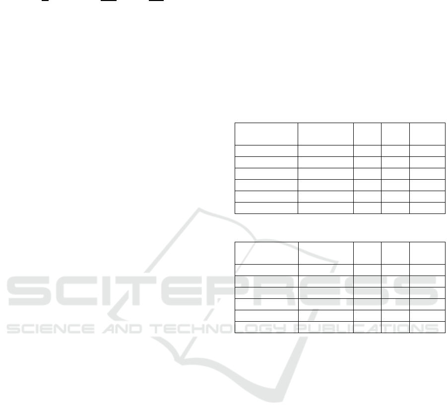
and EU (precisely Holland). The tested
configurations have had parameters presented in the
table 1 and the table 2. There were selected standard
configuration in view of its widespread use and
moderate cost.
Table 1: Tested configurations – GC virtual machines.
Config. name Vendor name No. of
CPUs
Loc-
ation
Price
[$/h]
GC-EU CPU-1 n1-standard-1 1 EU 0.0346
GC-EU CPU-2 n1-standard-2 2 EU 0.072
GC-EU CPU-4 n1-standard-4 4 EU 0.144
GC-US CPU-1 n1-standard-1 1 US 0.038
GC-US CPU-2 n1-standard-2 2 US 0.076
GC-US CPU-4 n1-standard-4 4 US 0.154
Table 2: Tested configurations – Azure virtual machines.
Config. name Vendor name No. of
CPUs
Loc-
ation
Price
[$/h]
Az-EU CPU-1 DS1 v2 1 EU 0.068
Az -EU CPU-2 DS2 v2 2 EU 0.136
Az -EU CPU-4 DS4 v2 4 EU 0.272
Az -US CPU-1 DS1 v2 1 US 0.07
Az -US CPU-2 DS2 v2 2 US 0.14
Az -US CPU-4 DS4 v2 4 US 0.279
The assumptions for the experiment was the
following:
 in each cloud three configurations CPU 1, CPU
2, and CPU 4, built with 1, 2, and 4 processor
virtual machines were used,
 four different loads were tested – the load task
executed by 25, 50, 100, and 200 users at once,
 there were performed series of measurements
during day (from 10:00 to 12:00 of local time)
and night (from 22:00 to 24:00 of local time),
 each series consisted of 50 to 200 probes
(requests for service for each service),
 for each probe there were collected various
parameters, among the others response time,
 for each series there were calculated various
parameters, among the other average response
time, percentiles, min value, max value, etc.,
 every measurement value was calculated from
values of 10 series (i.e. 500 to 2000 probes).
The evaluation of effectiveness with use of
proposed APPI index was performed for the index
A Cost based Approach for Multiservice Processing in Computational Clouds
435

parameters selected according to work (Everts, 2016),
i.e.:
 the satisfaction value equal 1,5 sec.
 the tolerance value equal 0,5 sec.
The assumption for the experiment was that the
measurements should be performed for processing
various types of tasks. As s measurement benchmark
the own Java based application was developed. The
task was run as a service which consists of the
following operations (9 available services):
1. AddData - adding a new object to the database.
2. AddUsr - adding a new user to the database with
password encryption,
3. AES - encryption and decryption of 10,000
bytes message using the AES algorithm with
256 bit encryption key length,
4. db1 – performing operation on database object,
5. db100 - reading 100 objects from the database
in JSON format (data size 44000 bytes),
6. Page - downloading static web page content of
size 1,9 MB,
7. Matrix – simple operation on matrixes,
8. Sort - performing a sorting algorithm for a set of
100000 elements,
9. TSP - resolving travelling salesman problem for
10 nodes (cities), 200 iterations, population size
50, and mutation 0,01,
After the measurements the evaluation Apdex
index and APPI index were calculated for all tested
configurations. These indexes can be considered to
choose the recommended environment for individual
processing needs. The APPI index was evaluated for
different acceptable prices P
AC
from 0,08 $/h (US
dollars per hour) to 0,3 $/h.
For more detailed service behaviour analysis the
recorded raw data of each measurement series was
used. Each and every value was calculated from
numerous series of probes executed in described real
cloud configurations with use of built mentioned
benchmark application.
3.1 General Evaluation of Processing
Environment
As the first step, the comparison of processing in real
clouds was performed without considering the
financial cost of processing using Apdex index.
Because no significant differences between
measurements during the day and the night were
observed, the results have been aggregated. In the
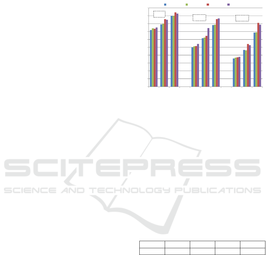
figure 1 the evaluation of effectiveness of processing
for the configurations located in EU and US for
CPU-1, CPU-2, and CPU-4 configurations, for load
L=50, 100, and 200 is presented.
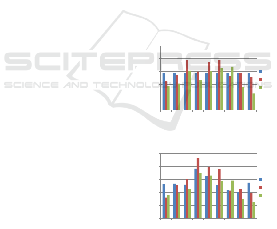
Figure 1: The evaluation of effectiveness of processing with
use of Apdex index for Google Cloud and Azure, in EU and
US, for configurations CPU-1, CPU-2 and CPU-4, and for
load L=50, 100, and 200.
The differences between location in EU and US
are small (however machines in US are usually
slightly faster). The machines in Azure are a little
more efficient, what is probably caused by using more
powerful equipment. The difference is larger for
larger load and when more CPUs are used. The only
discrepancy is for Az-EU CPU-2 configuration. It
seems that during this test something happened in
Azure cloud and processing performance decreased
globally in EU location. Detailed results show that it
happened for daily test. The standard deviation  of
measurements presented in the table 3 show that
results for Google Cloud are more stable in general.
Table 3: Standard deviation for aggregated measurements
in tested clouds, in EU and US.
Clou
d
GC-EU GC-US Az-EU Az-US

0,024 0,025 0,035 0,028
On the basis of collected measurements and the
cost of computing for each configuration the
effectiveness considering financial cost was
evaluated with use of APPI index. The assessment
was performed for various acceptable price. The two
examples are presented in the figure 2 and the figure
3.
0
0,1
0,2
0,3
0,4
0,5
0,6
0,7
0,8
0,9
1
CPU‐1CPU‐2CPU‐4CPU‐1CPU‐2CPU‐4CPU‐1CPU‐2CPU‐4
GC‐EU GC‐US Az‐EU Az‐US
L=50
L=100
L=200
ICEIS 2020 - 22nd International Conference on Enterprise Information Systems
436

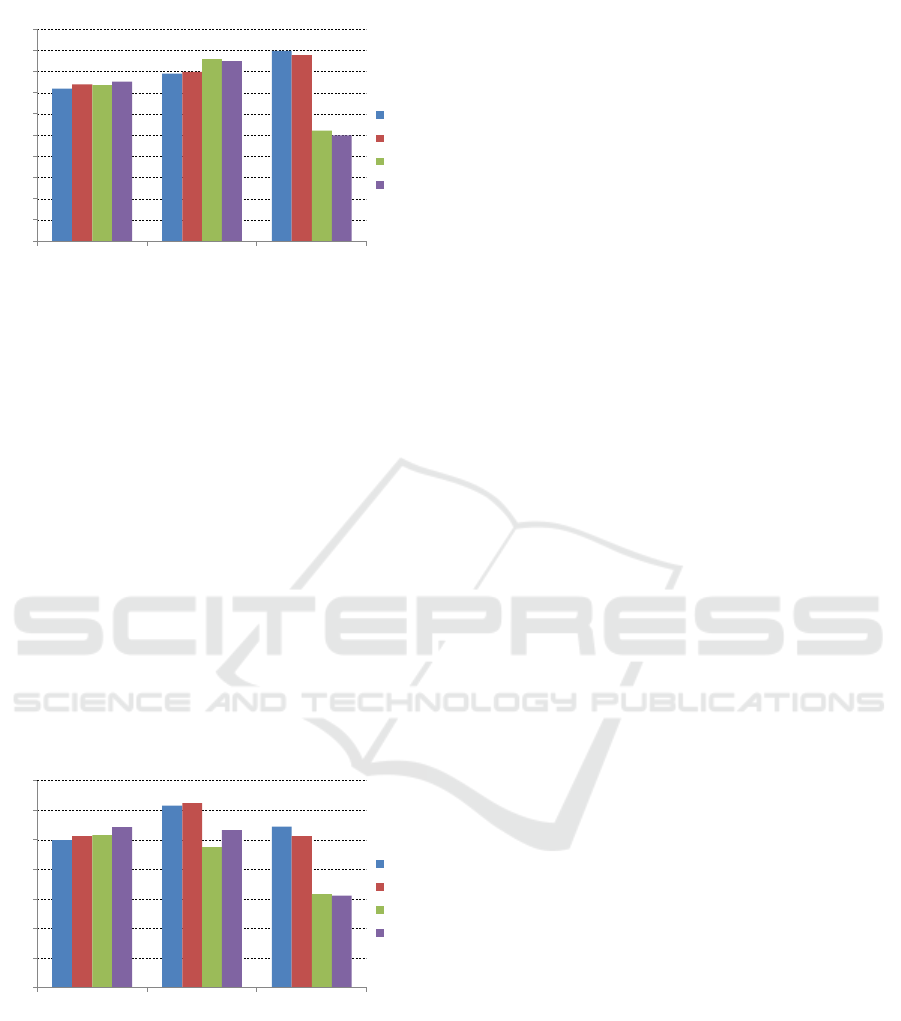
Figure 2: The evaluation of effectiveness of processing with
use of APPI index for Google Cloud and Azure, for
configurations CPU 1, CPU 2 and CPU 4, and for load
L=50,.and acceptable price P
AC
=0.15 $/h.
In the figure 2 are compared all configurations for
load L=50 and for acceptable cost of processing
P
AC
=0,15 $/h. While for no cost limit (using Apdex
index) almost in all cases the best solution for
processing was Azure, in this case the acceptable
price does not affect less expensive configurations
CPU-1 and CPU-2, and the choice is the same, but the
impact of price for configuration CPU-4 is obvious
and the cost limit now show strongly the GC-EU
configuration as the best solution.
In the figure 3 are compared configurations for
bigger load L=100 and for acceptable cost of
processing P
AC
=0,10 $/h. The lower acceptable price
now points to Google Cloud as recommended
solution for both configurations CPU-4 and CPU-2.
Figure 3: The evaluation of effectiveness of processing with
use of APPI index for Google Cloud and Azure, for
configurations CPU 1, CPU 2 and CPU 4, and for load
L=100,.and acceptable price P
AC
=0.10 $/h.
A noteworthy conclusion got from the figures 2
and 3 is that APPI index decreases evaluation of
effectiveness significantly, when the cost of
computing goes beyond the acceptable price. It raises
some doubts if this impact is not too strong.
3.2 Individual Service Analysis
The proposed APPI index can be used for general
selection of recommended cloud platform
configuration considering also acceptable price of
processing. But important drawback of this approach
is that may not have regard to individual type of
computations (services), especially when its
characteristics are significantly different. E.g., when
we looked deeper into measurements data, for an
example case – cloud environment GC-EU, CPU-4,
the load L=50 – the value of general indexes
Apdex=APPI=0,79, the value of Apdex index for
Matrix service is 0,56, for db100 service is 0,72 and
for TSP is 0,99. So the satisfactions of response times
are significantly different for each service.
In order to reflect efficiency of processing
requests for each service separately, having regard to
relations and changes of the load and cloud
configurations (i.e. available computing resources)
the relative response time RRT
u,l
determined for each
service in given processing conditions is defined as
specified in formula (2):

,

,
/


(2
)
where: u – is the service (application class) index,

,
– is average response time of service u under the
load l, 


– is assumed base value of response time
of given service u. All values are relative to 


and
allow compare relative increase or decrease of the
speed of processing.
The base response time can be chosen arbitrary
and for various purposes. In this paper, for the clarity,
the shortest average response time is used, i.e. the
time of processing in most powerful configuration
with the lowest load. It is worth to point out that 


is different for each service, hence one can clearly
compare behaviour of various services versus
configuration and load change, and relationships
between services.
For deeper analysis of processing efficiency the
measurements were performed for the following
environments and test cases: GC-EU cloud, CPU-1,
CPU-2, and CPU-4 configuration, the load L=25, 50,
and 100. The results were calculated from 9 series of
measurements (one most outlier series value was
dropped out).
In the figure 4, the figure 5, and the figure 6 the
relative response times RRT of each service and for
different loads are presented. There were tested 9
previously described services. The results are
presented for GC-EU configurations CPU-1, CPU-2
and CPU-4. The figure 4 presents the relative service
0
0,1
0,2
0,3
0,4
0,5
0,6
0,7
0,8
0,9
1
CPU‐1CPU‐2CPU‐4
APPI
LoadL=50,Acc.priceP
AC
=0,15
GC‐EU
GC‐US
Az‐EU
Az‐US
0
0,1
0,2
0,3
0,4
0,5
0,6
0,7
CPU‐1CPU‐2CPU‐4
APPI
LoadL=100,Acc.priceP
AC
=0,10
GC‐EU
GC‐US
Az‐EU
Az‐US
A Cost based Approach for Multiservice Processing in Computational Clouds
437

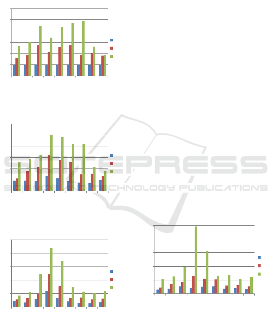
response times RRT for the load L=25, the figure 5
presents results for the load L=50, and the figure 6 for
the load L=100.
Figure 4: The relative service response times RRT for
GC-EU cloud, for configurations CPU-1, CPU-2 and
CPU-4, and for the load L=25.
Figure 5: The relative service response times RRT for
GC-EU cloud, for configurations CPU-1, CPU-2 and
CPU-4, and for the load L=50.
Figure 6: The relative service response times RRT for
GC-EU cloud, for configurations CPU-1, CPU-2 and
CPU-4, and for the load L=100.
The first important conclusion from the
experiments is that degradation of efficiency of
processing (here increase of the response time) is
different for different services in spite of using
consistent burden (the load benchmark was composed
of all services). E.g. for the load L=25 and CPU-4 in
the figure 4, the services 2 and 3 are processed 3 and
4,5 times slower respectively, or for the load L=50
and CPU-2 in the figure 5, the services 2 and 4 are
processed 3,5 and 6,5 times slower respectively. This
may not be a big surprise, however more interesting
is the second conclusion.
The degradation of efficiency of processing in
comparison to other service depends also on the load
– may be different for different loads. E.g. for the load
L=100 in the figure 6 the degradation of efficiency for
services 7 and 8 is similar. But for the load L=25 and
L=50 in the figure 4 and figure 5 respectively the
degradation for CPU-4 configuration is significantly
higher (almost twice) for service 7. It is not easy to
explain. Such behaviour can be caused by specific
combination of available different resources (CPU,
memory, backend support (e.g. database support),
etc.) and different demands for such resources by
each service (application).
In the figure 7 the relative service response times
RRT for the load L=25, L=50, L=100, for one
configuration CPU-2 is presented. It can be noticed
how specific services differs regarding processing
efficiency degradation for different system load.
Again, the differences depend not only on services
but also on current system load. The general
characteristic of service behaviour was similar for
other configurations i.e. CPU-1 and CPU-4.
Figure 7: The relative service response times RRT for
GC-EU cloud, for configuration CPU-2, and for the load
L=25, L=50, and L=100.
The general conclusion is that for effective
selection of cloud configuration according to any
criteria that take into consideration also response
0
1
2
3
4
5
6
123456789
RRT
u
LoadL=25
CPU‐4
CPU‐2
CPU‐1
0
2
4
6
8
10
12
123456789
RRT
u
LoadL=50
CPU‐4
CPU‐2
CPU‐1
0
10
20
30
40
50
123456789
RRT
u
LoadL=100
CPU‐4
CPU‐2
CPU‐1
0
5
10
15
20
25
123456789
RRT
u
CPU‐2
25
50
100
ICEIS 2020 - 22nd International Conference on Enterprise Information Systems
438

time, one needs a characteristics of the configuration
for each of considered types of application and for
every different loads one has to count.
4 CONFIGURATION SELECTION
APPROACH WITH REGARD
TO PROCESSING COST
In this paper the case of cloud environment in which
different services are run at the same time, is
considered. As stated in previous section, to develop
any approach to manage processing in such a case
with regard to service response time one should use a
parameter characterizing each cloud configuration for
each considered type of service and for each load it
should be taken into consideration. In presented case
such parameter is RRT
u,l
i.e. relative response time for
the service u and the load l, calculated according to
formula (2) for each tested load, and derived on the
basis of values obtained from the performed
benchmark.
Having several cloud configuration alternatives
additional demands related not only to processing
time efficiency but also to processing cost, can be
stated. Here two elementary cases are discussed: 1)
how to reduce absolute processing cost, and 2) how
to reduce processing cost with regard to satisfy
quality of user experience expressed with use of
response time. Both use relative response time RRT
u,l
.
The first approach is related to the problem of
running a service such as it is processed as cheap as
possible what can be defined as the following: a
multiple of time of processing and price for using
cloud configuration per time is the lowest. As
presented in previous section the time of processing
depends on the configuration, but also on general
load, and its changes are not proportional, so the
choice is not obvious. In this approach we propose to
use relative processing cost RC determined with use
of RRT from the benchmark, and with use of price of
given cloud configuration.
Let 


be the cloud configuration price (virtual
machine price) of m-th configuration. For the given
m-th configuration the relative processing cost
parameter 
,

that characterizes relative change of
price cost of processing for given service, and for
given load is determined with formula (3):

,




/
,


(3)
where 
,

is relative response time of service u
with load l for configuration m.
The rule defined to choose the configuration is the
following:

,
∗
←argmin


,

(4
)
where 
,
∗
- is the chosen configuration m for the
given service u and the load l.
The presented method requires determination of
RC values for loads that can be expected. The
simplest approach to use the presented procedure is
assuming the specific values of the load L (l=L
1
, l=L
2
,
etc.) that can be maximally allowed and determine the
configuration for these values.
The chosen configuration that minimizes the
value of relative processing cost 
,

can be
different not only for different services, but also may
vary with load change. The figures 8 and 9 present the
relative processing cost calculated from the results of
test benchmark run in real cloud environments (GC-
EU) for 9 tested services, for two loads L=25 and
L=50 (each for CPU-1, CPU-2, and CPU-4).
Figure 8: Relative processing cost for GC-EU, for confi-
gurations CPU-1, CPU-2 and CPU-4, for the load L=25.
Figure 9: Relative processing cost for GC-EU, for confi-
gurations CPU-1, CPU-2 and CPU-4, for the load L=50.
0
0,05
0,1
0,15
0,2
0,25
123456789
RC
LoadL=25
CPU‐4
CPU‐2
CPU‐1
0
0,1
0,2
0,3
0,4
0,5
123456789
RC
LoadL=50
CPU‐4
CPU‐2
CPU‐1
A Cost based Approach for Multiservice Processing in Computational Clouds
439

Because the assumed base value of response time
was the average response time for configuration
CPU-4 and for the load L=25, for this case the relative
processing cost RC is a reference value and is equal
for all services (they are only used for relative
comparison processing cost for the given service and
the given load when different configurations are
considered).
It can be noticed that for the load L=25 for service
8 the best choice is configuration CPU-1 (next CPU-2
or CPU-4 – almost the same value). Similarly, for the
load L=50 (here CPU-4 is a little better than CPU-2).
In contrast, for the service 3, for the load L=25 the
best choice is configuration CPU-4 (next CPU-1
(slightly worse) and CPU-2 (significantly worse)),
but for the load L=50 the situation changes – the best
is configuration CPU-1 (the configuration CPU-2 is
still the worse).
The second approach takes into consideration not
only the demand to choose the best configuration in a
sense of first approach, but also the demand to satisfy
one of the most often specified quality of user
experience parameter - the maximal service response
time. Here, for simplicity, the average response time
is considered.
Let define for each service u the required average
response time T
u
= k
u
T
u
BRT
– this parameter is
specified for each service relatively to base response
time (here it is the time of processing in most
powerful configuration with the lowest load). Having
determined relative service response times RRT and
relative processing costs RC for services u and
considered loads the choose of preferred
configuration for running given service is performed
the same according to formula (4) with respect to
additional condition (5):

,



(5)
Again, the simplest approach to use the procedure
is to assume specific values of maximally allowed
load l=L and determine the configuration for these
values. This especially makes sense because usually
one wants to satisfy service quality with worst
allowed processing conditions (maximally allowed
load) and for lower loads the average time of
processing is not higher for given configuration.
Putting the above together, for our measurements
in real cloud configurations an example of using the
approach is the following:
‒ let consider service u=8 (Sort application),
‒ assume required response time T
7
=3.5T
7
BRT
(it
is 3.5 times greater than base response time),
‒ for the load L
1
=25 the calculated values of
parameters are the following:

,

2,60 for m
1
(CPU-1),

,

2,01 for m
2
(CPU-2),

,

1,00 for m
3
(CPU-4)
– all configurations are allowed (for all
RRT<3.5) – see the figure 4,
‒ for the load L
1
=25:

,

0,090 for m
1
(CPU-1),

,

0,145 for m
2
(CPU-2),

,

0,144 for m
3
(CPU-4)
– the minimum is for configuration CPU-1 – see
the figure 8,
‒ for the load L
2
=50:

,

4,35 for m
1
(CPU-1),

,

3,12 for m
2
(CPU-2),

,

1,39 for m
3
(CPU-4)
–configuration CPU-1 is not allowed (it is too
slow) – see the figure 5,
‒ for the load L
2
=50:

,

0,225 for m
2
(CPU-2),

,

0,201 for m
3
(CPU-4)
– the minimum is for configuration CPU-4 – see
the figure 9.
For the required response time the choices are CPU-1
for the load L=25 and CPU-4 for the load L=50.
5 FINAL REMARKS
The paper focuses on issues related to evaluation of
processing environment for cloud computing. The
goal of presented study was to investigate potentiality
for assessment of processing in selected
computational clouds taking into consideration the
response time and financial cost constraints.
The base of proposed approach is the relative
response time RRT determined from load test
benchmark, calculated for some selected base
response time value, and for each service separately.
It enables to characterize the behaviour of
individual services under different processing
conditions. Presented results of experiments
performed in real clouds show that for effective
selection of cloud configuration according to criteria
that take into consideration also response time, while
different types of services (applications) are used, a
characteristic related to each of considered types of
application, and for every load one has to count is
needed. Such parameter RRT is quite easy to use and
for given prices of available cloud virtual machine
configurations enables to choose target machine to
run the application with regard to considered
ICEIS 2020 - 22nd International Conference on Enterprise Information Systems
440

demands, including service response time and price
cost.
However, the proposed approaches have same
limitations. Among the others it is assumed that the
load has uniform characteristic. In presented case the
number of requests performed at the same time for
different services was proportional for each service.
On the whole the situation can be different. Different
services may consume environment resources
differently and then the impact on RRT of given
service can vary. So, the determined values of RRT
(and consequently relative cost RC) may not be
always precise enough. Here, the further extension for
presented approach is desirable.
REFERENCES
Al-Said Ahmad A., Andras P., 2019, Scalability analysis
comparisons of cloud-based software services,
available at https://doi.org/10.1186/s13677-019-0134-
y, Springer Open.
Aminm F., Khan, M., 2012, Web Server Performance
Evaluation in Cloud Computing and Local
Environment, Master’s Thesis, School of Computing
Blekinge Institute of Technology
Autili M., Di Ruscio D., Inverardi P., Tivoli M.,
Athanasopoulos D., Zarras A., Vassiliadis P.,
Lockerbie J., N. Maiden N., Bertolino A., De Angelis,
G., Ben Amida A.,, Silingas D., Bartkeviciu R., Ngoko
Y.,, 2011, CHOReOS Dynamic Development Model
Definition (D2. 1), Technical report.
Becker M., Lehrig S., Bccker S., 2015, Systematically
Deriving Quality Metrics for Cloud Computing
Systems, CPE’15: Proceedings of the 6
th
ACM/SPEC
International Conference on Performance
Engineering, pp. 169-174, available at
https://doi.org/10.1145/ 2668930.2688043.
Chen, T., Bahsoon, R., 2015 Toward a Smarter Cloud: Self-
Aware Autoscaling of Cloud Configurations and
Resources, Computer 48(9), 93 - 96.
Dhall, C., 2018, Scalability Patterns - Best Practices for
Designing High Volume Websites. 1st edn, Apress.
Everts, T., 2016, Time Is Money - The Business Value of
Web Performance, 1st edn, O'Reilly Media Inc.
Fras M., Kwiatkowski J., Stas M., 2019, A Study on
Effectiveness of Processing in Computational Clouds
Considering Its Cost, Information Systems Architecture
and Technology: Proceedings of 40th Anniversary
International Conference on Information Systems
Architecture and Technology – ISAT 2019, Springer
Nature Switzerland AG 2020, pp. 265-274.
Fraczek, J., Zajac, L., 2013, Data processing performance
analysis in Windows Azure cloud, Studia Informatica,
vol. 34, no 2A, 97-112.
Habrat, K., Ladniak, M., Onderka, Z., 2014, Efficiency
analysis of web application based on cloud system.
Studia Informatica, vol. 35, no. 3, 17–28.
Kaminska, M., Smihily, M., 2018, Cloud computing -
statistics on the use by enterprises, https://ec.europa.eu/
eurostat/statistics-explained/index.php/.
Lehrig S., Eikerling H., Becker S., 2015, Scalability,
Elasticity, and Efficiency in cloud Computing: a
Systematic Literature Review of Definitions and
Metrics, Proceedings of the 11th International ACM
SIGSOFT Conference on Quality of Software
Architectures, pp. 83 – 92.
Leitner, P., Cito, J., 2016, Patterns in the Chaos – a Study
of Performance Variation and Predictability in Public
IaaS Clouds. ACM Transactions on Internet
Technology, Vol. 6, Issue 3.
Popescu, D. A., Zilberman, N., Moore, A.W., 2017
Characterizing the impact of network latency on cloud-
based applications performance. Technical Report
Number 914, University of Cambridge - Computer
Laboratory, https://www.cl.cam.ac.uk/techreports/
UCAM-CL-TR-914.pdf.
Sevcik, P., 2005, Apdex interprets app measurements.
Network World, https://www.networkworld.com
/article/2322637/apdex-interprets-app-
measurements.html.
Shankar, S., Acken, J. M., Sehgal, N. K., 2017, Measuring
Performance Variability in the Clouds., 2018. IETE
Technical Review 35(6) 1-5.
Staś, M., 2019, Performance evaluation of virtual machines
in the computing clouds. Master’s Thesis, Wroclaw
University of Science and Technology.
Weins K., 2017, Cloud Computing Trends: 2017 State of
the Cloud Survey, available at https://www.rightscale.
com/blog/cloud-industry-insights/cloud-computing
-trends-2017-state-cloud- survey.
A Cost based Approach for Multiservice Processing in Computational Clouds
441