Fuzzy Gradient Control of Electric Vehicles at Blended Braking with

Volatile Driving Conditions

Valery Vodovozov

, Eduard Petlenkov

, Andrei Aksjonov

and Zoja Raud

Department of Electrical Power Engineering and Mechatronics, Tallinn University of Technology,

Ehitajate tee 5, Tallinn, Estonia

Department of Computer Systems: Centre for Intelligent Systems, Tallinn University of Technology,

Ehitajate tee 5, Tallinn, Estonia

School of Electrical Engineering, Intelligent Robotics Group, Aalto University, Espoo, Finland

Keywords: Electric Vehicle, Intelligent Transportation, Fuzzy Control, Modelling, Simulation, Energy Recovery,

Hybrid Energy Source, Braking System.

Abstract: The paper is devoted to intelligent control of road electric vehicles aiming at reducing energy losses caused

by traffic jams, changing velocity, and frequent start-stop modes of driving. A blended braking system is

described that integrates both the friction and the electric braking strengths in volatile driving conditions,

including gradual and emergency antilock braking. The vehicle model reflects multiple factors, such as air

resistance, road slope, and variable friction factor. A new gradient control method recognizes unstable tire

properties on changing road surfaces at different velocities. In the motor and battery model, the state of charge

and electric current/voltage restrictions of the hybrid energy storage are taken into account. The braking torque,

actuated by the Mamdani’s fuzzy logic controller established in the Simulink

environment, is allocated

between the front and rear friction and electric brakes. Comparison of simulation and experimental results

confirms that the outcomes of this research can be considered in the design of braking systems for electric

vehicles with superior energy recovery.

1 INTRODUCTION

In development of control systems for road electric

vehicles, many novel energy saving trends are

discovered nowadays. In view of the fact that up to

50 – 70% of vehicle energy is lost during deceleration

(Shang et al., 2010; Savaresi et al., 2010), the braking

energy recovery might reclaim this loss and extend

driving range and time. Thereby, the introduction of

modern blended braking systems has become a top

priority and moves forward intensively in recent

years. Such systems combine traditional friction

braking (FB) with regenerative electric braking (EB)

associated with hybrid energy storage machinery that

unites both high energy density modules (batteries)

and high power density blocks (ultracapacitors or/and

flywheels) (Naseri et al., 2017). Blended braking has

https://orcid.org/ 0000-0002-5530-3813

https://orcid.org/ 0000-0003-2167-6280

https://orcid.org/ 0000-0001-7460-6548

https://orcid.org/ 0000-0001-5197-3599

attracted attention in science and industry because of

reduced car maintenance costs and lowered tire

particles emission, among others.

Most electric vehicle designers, such as (Chen et

al., 2017; Xie and Wang 2018), prefers EB for vehicle

gradual slowing down and FB for intensive

deceleration. EB is commonly out of use in the

antilock braking system (ABS) and is not applied as

an urgent braking tool because the force generated by

an electric motor is often quite small to produce the

total braking torque needed to ensure a quick and

steerable stop. Primarily, the EB fails due to battery

overheating and the state-of-charge (SOC)

restrictions of the energy storage.

When discussing the distribution of braking

torque in blended braking systems, three approaches

fall to the focus of attention: force assignment

250

Vodovozov, V., Petlenkov, E., Aksjonov, A. and Raud, Z.

Fuzzy Gradient Control of Electric Vehicles at Blended Braking with Volatile Driving Conditions.

DOI: 10.5220/0009777602500261

In Proceedings of the 17th International Conference on Informatics in Control, Automation and Robotics (ICINCO 2020), pages 250-261

ISBN: 978-989-758-442-8

between right and left wheels, power sharing among

front and rear wheels, and torque allocation between

EB and FB systems (Xu et al., 2016). The last issue is

aimed at acquiring maximal braking energy from both

EB and FB ensuring highest regeneration capacity

and involving the EB to energy exchange in the best

possible way (Xie and Wang, 2018). At that, the ABS

occupies a special place and usually represents a

separate part of the vehicle, since its primary target is

to reduce the braking distance and time.

Usually, ABS performs poorly in volatile and

unknown road conditions because of its focus on

high-speed driving on straight dry roads. As a result,

when rain, snow, or loose gravel appears, ABS can

lengthen the braking distance and braking time

instead of shortening them due to improper control

organisation. To resolve the problem, intelligent

ABSs with slip adjustment were proposed (Naseri et

al., 2017; Chen et al., 2017).

For the systems that have non-linear and time

variant plants with significant dead time, multiple

fuzzy control approaches were published recently.

Thanks to such universal approximator as a fuzzy

logic controller (FLC), the most progressive of them,

for instance (Givigi, 2010; Haidegger, 2011),

successfully evaluate a priori unknown changes in the

environment over time in order to understand the

process and to find a solution of the dynamic

differential or difference equations. In (Radgolchin,

2018), a fuzzy controller is designed to stabilize a

moving plant at unknown deflections. The efficiency

of this FLC is enhanced using a second level

supervisory controller. The fuzzy algorithm proposed

in (Precup, 2014) computes the control signal vector

applied to the chaotic continuous-time dynamical

system to ensure its stabilization.

In (Lin and Song, 2011), changes in the properties

of tires, road surfaces, and vehicle deceleration can be

estimated taking into account the displacement and

rate of the brake pedal pressing, vehicle velocity, and

wheel slip as the FLC input signals. Nevertheless, this

specifity eliminates the use of EB in the ABS and

separates the ABS from the general braking system.

As a rule, while the braking intensity demand is small,

EB is elected, but as the ABS is requested, FB is

applied (Jing et al., 2011).

Just like in the initial part of this research

published in (Aksjonov et al., 2018; Aksjonov et al.,

2019), the current study is devoted to creating a

hybrid energy-storage-oriented blended braking

system suitable for different braking modes on

various road surfaces and velocities. However, new

factors are taken into account here aiming at

improving the efficiency of energy recovery and the

versality of the system. First, thanks to the torque

gradient control, the available range of volatile

driving conditions is expanded without losing the

quality of braking. Second, in addition to ABS, the

offered braking system can operate in both gradual

and emergency braking modes. Third, in contrast to

many known ABS, the quality of braking in this study

does not depend on the initial vehicle velocity, air

resistance, or road incline.

The problem of braking management is

formulated as a search among three actions: urgent

braking with fuzzy ABS control upon maximally

possible EB involvement; gradual braking with

greatest energy recovery; or non-electric braking. The

research objective is to achieve the best energy

recovery in the first two scenarios with minimal

participation of the third one. The following five

sections present the new braking system with gradient

control, the vehicle friction model, the motor-battery

model, and their operation. Then, the versatile

braking FLC is designed. Next, the simulation is

performed, the experimental diagrams are compared

to the simulation outcomes, and the results obtained

are summarized.

2 MODEL OF BRAKING SYSTEM

In compliance with (Reif, 2014; Kiyakli and Solmaz,

2018), dynamics of the braking single-wheel quarter-

vehicle are determined as follows:

Fma



, (1)

= F

air

, (2)



 

windvwindvairair

vvvvQCF  sgnρ5.0

, (3)



βsinmgF



(4)



β cos μ mgF



, (5)

JrFT



, (6)

where

m – quarter-vehicle mass;

a – longitudinal deceleration of vehicle;

– braking force;

air

– air resistance (aerodynamic drag);

ρ – air density;

air

– aerodynamic drag coefficient;

Q – vehicle front area;

= – vehicle velocity;

wind

– wind velocity;

Fuzzy Gradient Control of Electric Vehicles at Blended Braking with Volatile Driving Conditions

251

– climbing force;

g – acceleration due to gravity;

β – climbing slope (road incline);

– longitudinal force;

μ – dimensionless friction factor;

– braking torque;

r – effective radius of the wheel;

– angular speed of the wheel;

J – moment of inertia of the wheel.

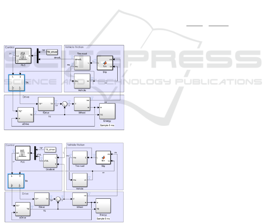
Two variants of the explored Simulink

model of

blended braking with fuzzy gradient control are

shown in Fig. 1: the friction-slip system (a) and the

torque-slip system (b). They are made up of the

following groups of blocks:

• Vehicle friction group including Tire-road, Slip,

and Vehicle blocks;

• Drive group, including electric drive (eDrive),

friction drive (fDrive), Wheel, and Energy blocks;

• Control group, including the fuzzy logic

controller (FLC) and torque allocation (TA)

blocks. The FLC derives an actuating braking

torque T

for vehicle deceleration using the

velocity and tire-road (a) or application torque (b)

gradient signals.

(a)

(b)

Figure 1: Simulink

models of the blended braking system

with friction-slip (a) and torque-slip (b) gradient control.

3 WHEEL SLIP AND TIRE-ROAD

FRICTION ESTIMATES

To slow down the vehicle moving at certain initial

velocity v

, the required braking force F

has to be

developed. To this aim, the control system needs the

data used in Eqs. (1) – (6). Most of them are available

from the vehicle passport characteristics (m, Q, r, J)

or can be acquired with on-board sensors (a, v

wind

, ω

However, estimating the total tire-road friction is

a complex challenge since this parameter varies with

such factors as velocity, load, torque, surface

roughness, tire diameter, inflation, wear, etc., and

these variations are very difficult to detect. Moreover,

the friction depends on the wheel slip.

Unlike the graduate braking, in intensive braking

a longitudinal wheel slip λ takes place (Reif, 2014;

Spichartz et al., 2017) i.e. the relative difference

between vehicle (v

) and wheel (v

) velocities:

vv ω









. (7)

This means that in addition to minor rolling

friction, slipping friction heavily affects the braking

rate. It involves both the kinetic interaction of moving

surfaces, called sliding or dynamic friction, and the

static coupling (“stiction”) of fixed surfaces. The

latter one significantly exceeds its kinetic counterpart

at the beginning of starting and at the end of braking.

The force that prevents a tire from slipping as it rolls

on the ground is an example of static friction. Even

though the wheel is in motion, the patch of the tire

that contacts the ground is stationary relative to the

ground, so it is a static rather than a kinetic fraction

(Pratap and Ruina, 2002).

To derive the wheel slip in real time, both

velocities in Eq. (7) can be directly measured with on-

board v

and ω

sensors. However, since the friction

cannot be acquired by sensors, one or the other

computational method is required for its estimation.

The knowledge of the friction-slip characteristics





v,λμ

is needed not only to ensure the anti-spin

regulation and antilock braking, but also, for adaptive

cruise control and energy recovery. As direct friction

sensing is impossible, many studies devoted to its

indirect estimation have been produced aiming to

arrange the braking procedure. In all cases, some

forms of the model-based approach are used for





v,λμ

searching. In (Zhang and Lin 2018), friction

is derived based on velocity sensor signals and

vehicle geometry. In (Kadowaki et al., 2007), a

ICINCO 2020 - 17th International Conference on Informatics in Control, Automation and Robotics

252

perturbed sliding mode observer is used. Several

models of the friction-slip relations may be found in

literature, such as Pacejka’s “Magic Formula”,

Burckhardt model, Rill model, and others (Cecotti,

2012).

Although the factors in these models are different,

the trends of curves look very similar. Commonly, the

tire-road friction factor grows steeply from zero to its

maximum appeared somewhere between 2 and 12%

slip for different road surfaces. At 0% slip, both the

wheel and the vehicle have exactly the same

velocities in Eq. (7). Gradual braking operations

presume low levels of slip and take place within a

zone where an increase in the slip simultaneously

produces an increase in the usable friction. These

growing slopes of the friction-slip characteristics

match the stable zone where, due to the positive

friction-slip gradient, the vehicle is suitable for

control and for steerability maintenance. On the

contrary, the falling slopes emphasise an unstable

zone, in which the wheels may lock up, inducing

skidding and causing the spinning of the tires. When

the slip is 100%, the wheel is locked although the

vehicle is still moving.

In this research, a programmable road estimator

was implemented in the Tire-road block shown in

Fig. 1, where a preliminary stored set of friction-slip

lookup tables is used. Its input is associated with the

Slip block and vehicle deceleration a is derived from

the ratio of the longitudinal (F

) and normal (F

)

forces acting on the wheel:



β cos

,λμ

FFma

gair





. (8)

Further, vehicle velocity is counted by integrating

a as shown in Fig. 2, where it is assumed that F

air

= β

= 0 with a view to simplicity.

Figure 2: The Vehicle block.

Naturally, given the very large uncertainty

associated with the above estimates due to incomplete

data, this approach does not claim to be highly

accurate. As the velocity decreases, the curves tend to

move down and right, meaning that the dynamics of

the wheel slip is inversely proportional to the vehicle

velocity (Habibi and Yazdizadeh, 2010; Cerdeira-

Corujo et al., 2016; Li et al., 2018). Additionally, such

tire properties as their type, inflating pressure, etc.

also change during braking, affecting their peak

locations. An important challenge is to identify the

changing road surface in order to select the proper





v,λμ

characteristic.

4 GRADIENT CONTROL

METHOD

In contrast to (Aksjonov et al., 2018), where the

acceleration signal is sent directly to the controller, in

the new model presented in Fig. 1 this signal is only

needed to estimate the vehicle velocity in the Vehicle

block.

To reduce the uncertainty of the friction

characteristics, the steerable braking condition can be

confidently expressed as



. (9)

In accordance with Eq. (9), the fastest braking

process is expected at the maximal braking force F

corresponding to



In the model of Fig. 1-(a), the desired friction

factor and the measured slip ratio are used in the same

Tire-road block to determine how great force can be

created in response to an increase of wheel slip.

Estimation of Eq. (9) in real time is based on the

tire model Eq. (8). Two approaches are proposed to

overcome differentiation noise. In the first case, a

filtering technique (Cecotti et al., 2012) is adopted.

As the second method, pre-calculated friction

derivatives are collected in the lookup tables to be

used instead of real-time differentiation. The gradient

obtained by any of these approaches is further

directed to the control system.

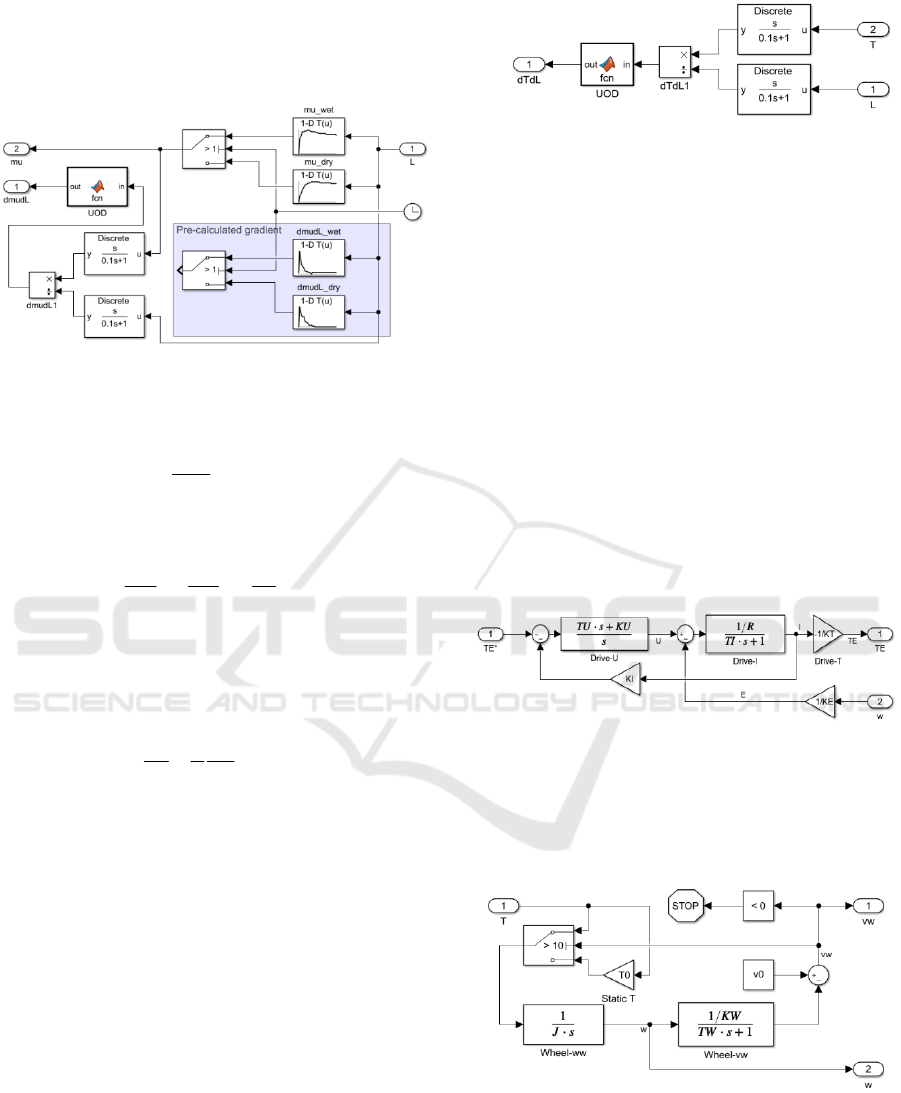
Both techniques are illustrated in Fig. 3, where

two lookup tables keep data on the friction-slip (mu-

L) relations on wet (mu_wet) and dry (mu_dry) roads,

and two other lookup tables (dmudL_wet and

dmudL_dry) keep data on the pre-calculated

gradients. The signals about the change of the road

surface connect the appropriate tables to the outputs

of the block. At that, the derivatives are restricted

according to the universe of discourse (UOD) of the

connected controller.

Management of braking using Eq. (9) is called

further a friction-slip gradient control. Since friction

cannot be sensed directly and this control approach

Fuzzy Gradient Control of Electric Vehicles at Blended Braking with Volatile Driving Conditions

253

remains fairly rough, the estimated tire-road friction

factor is to be taken with a margin relative to its

maximum. As a result, this system does not claim any

significant advantages over (Aksjonov et al., 2018).

Figure 3: The Tire-road block.

However, as a development of this approach, a

more advanced method is further proposed.

Assuming that

remains rather constant in

the controller computational interval, Eq. (6) can be

converted as

λλ d



, (10)

where



βcosmgrk 

In turn, since at the steerable braking the torque T

follows the application torque T of the drive, Eq. (9)

is re-written as follows:



. (11)

Now, the derivative of application torque with

respect to slip may be used as a control feedback. It is

called further a torque-slip gradient control.

Whereas the application torque is easily measured

with sensors and accurately adjusted (Xu et al., 2016),

the torque-gradient control represents a kind of the

close loop control. In this way, vehicle velocity,

particularly at statics, as well as other road,

aerodynamics, and incline features are successfully

considered into the tire model as was recommended

in (Habibi and Yazdizadeh, 2010; Cecotti et al.,

2012).

The torque-slip gradient control is illustrated in

Fig. 1-(b) and Fig. 4, where the Gradient block

implements differentiation of measured application

torque T, whereas the Tire-road block is only needed

for estimating the friction using data from the Slip

block fed by the on-board v and ω

sensors.

Figure 4: The Gradient block.

5 DRIVE MODEL

In the Drive group, the friction drive fDrive block,

integrated with FB, and the adjustable electric drive

eDrive block, implemented the battery-regenerative

EB, handle separately their portions of the actuating

braking torque T

generated by the Control group.

The FB unit is modelled as a first order system

with dead time.

In turn, the Drive-U sub-block in eDrive (Fig. 5)

is responsible for direct torque control, electrical

power supply, and energy recovery. Together with the

Drive-I sub-block, it arranges a torque stabilisation

loop with PI current controller.

The Drive-T sub-block and the Wheel block

belong to the speed loop activated in gradual

deceleration and shorted in emergency braking.

Figure 5: The eDrive block.

Gear and vehicle inertia are represented by the

Wheel block also (Fig. 6). The static fraction of torque

is taken into account in this model when the velocity

drops to a low (v

home

) level.

Figure 6: The Wheel block.

The Energy block (Fig. 7) derives an electrical

fraction of the braking power

wEE

TP ω



(12)

ICINCO 2020 - 17th International Conference on Informatics in Control, Automation and Robotics

254

and braking energy regenerated back to the supply

grid with efficiency η in a given time interval t:



 dtPW

(13)

Figure 7: The Energy block.

6 TORQUE ALLOCATION

The main mission of the blended braking system is to

slow down a vehicle under the action of the

application torque T, which should be as close as

possible to the driver’s setpoint T

(the block

TB_driver in Fig. 1), without exceeding peak

optimality for the road surface under the tires.

The Control group generates actuating braking

torque T

dependently of the pedal displacement T

and friction gradient dμ/dλ (Fig. 1-(a)) or application

torque gradient dT/dλ (Fig. 1-(b)). Its output torque

allocation block (TA) algorithmically distributes the

actuating braking torque T

between the front and rear

wheels in a fixed ratio (Tao et al., 2017) and allocates

it between FB and EB based on real-time SOC,

voltage, and permissible EB current. Electric current

recharges the energy storage device from the EB

while the pressure signal p

adjusts the FB. Braking

will complete when the driver releases the pedal or

the vehicle stops.

In order to forward to EB a maximal fraction of

the actuating torque T

, the electric drive has to

develop sufficient power, voltage, and current to

charge all energy storage devices:



max max max

,max

BATUCE

III

UUU

PPP



, (14)

where

UC max

, U

UC max

, I

UC max

, P

BAT max

, U

BAT max

, and

BAT max

are permissible power, voltage, and current of

the ultracapacitor (UC) and the battery (BAT),

respectively; P

E max

, U

E max

, and I

E max

– maximal

power, voltage, and current of the electric drive.

Meanwhile, in order to keep the battery and

ultracapacitor within their safe operating areas,

electric current I

and motor torque T

have to meet

the real-time storage restrictions, namely, SOC

and

SOC

BAT

(Cerdeira-Corujo, 2016; Naseri et al., 2017):

 



ψ ψ, max

BATBATUCUC

SOCISOCI

IT 

(15)

where I

and I

BAT

are estimated charging currents of

the ultracapacitor and battery and ψ is flux linkage of

the electric motor.

Once the actuating braking torque exceeds these

boundaries, the remaining part of it must be created

by the FB:

***

TTT 

. (16)

In (Aksjonov et al., 2019), an appropriate torque

allocation algorithm is proposed. There, when the

control system recognises the actuating torque

request T

, the EB is activated and either EB

BAT

runs. The FB torque does not appear until

either any of the SOC levels exceeds the allowed

overcharging barriers or the electric motor produces

maximal power. As soon as the motor torque becomes

insufficient, the system runs FB and EB together.

Only in the case when both SOC levels exceed their

boundaries, the solo FB is used due to the inability to

regenerate.

Therefore, the common trait of this strategy is to

include regeneration into all braking scenarios, even

during heavy braking with ABS, and to use the solo

FB only when the battery SOC and voltage levels are

saturated. The fewer such conditions appear, the less

braking energy is wasted and the longer the service

life of the FB.

7 DESIGN OF A FUZZY LOGIC

CONTROLLER

Depending on the solution chosen, the fuzzy (Tao et

al., 2017), PID (Cerdeira-Corujo et al., 2016; Kiyakli

and Solmaz, 2018), sliding (Kadowaki et al., 2007;

Habibi and Yazdizadeh, 2010), and some other

braking controllers compete in the market. Given the

complexity of the system and its nonlinearity, this

study is devoted to the FLC relying on the knowledge

and skills of professional experts.

The FLC target is to derive an actuating braking

torque T

needed for slowing down the vehicle inside

an acceptable friction-slip region. In the MISO-type

controller designed, two input numerical variables

(crisps) are used: the driver’s setpoint T

and either

the friction (dμ/dλ) or the application torque (dT/dλ)

derivative with respect to slip λ.

The Mamdani-style inference mechanism is

applied to transform every input crisp into a separate

fuzzy pair consisting of an element in UOD and an

Fuzzy Gradient Control of Electric Vehicles at Blended Braking with Volatile Driving Conditions

255

appropriate membership function (MF). The

estimated actuating torque T

is coming from the FLC

output. Using the weighted average defuzzification

method, this linguistic signal is then turned back to

the real-world output crisp.

The setpoint torque input T

, the gradient input

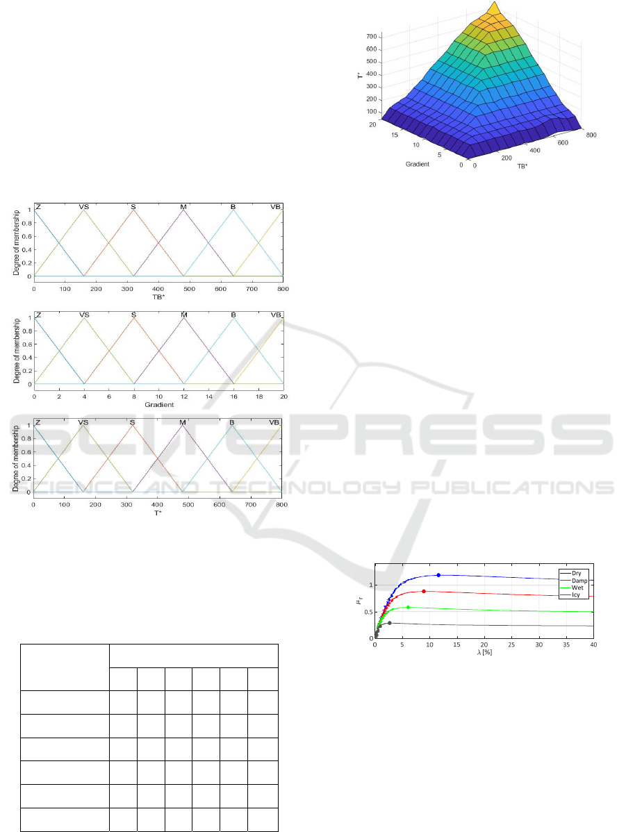
dT/dλ (or dμ/dλ), and the actuating torque T* output

have six MFs notated as Z (Zero), VS (Very Small),

S (Small), M (Middle), B (Big), and VB (Very Big).

In Fig. 8, the fuzzy sets for the linguistic variables

are represented. The MFs have a triangle shape

suitable for braking management and experts training.

Figure 8: MFs of control variables T

*, Gradient, and T*.

The inference engine with “If–Then” modus

ponens converts fuzzy input sets to the fuzzy output

set using the base of 36 rules shown in Table I.

Table 1: FLC Rule Base.

Gradient

dµ/dλ, dT/dλ

Output torque T* at input T

Z VS S M B VB

Z Z Z Z Z Z Z

VS Z VS VS VS VS VS

S Z VS S S S S

M Z VS S M M M

B Z VS S M B B

VB Z VS S M B VB

The input-output FLC surface is plotted in Fig. 9.

Figure 9: Input-output FLC surface.

8 EXPERIMENTATION

To validate the model described in the previous

sections, the simulations are compared further to

experimental results published in (Aksjonov et al.,

2019).

The hardware-in-the-loop electro-hydraulic

testbed from ZF TRW Automotive (Koblenz,

Germany) granted for experimentation by TU

Ilmenau (Germany) and driven by the vehicle-

oriented software IPG CarMaker

(Karlsruhe,

Germany) was used there. The detailed stand

specification is given in (Aksjonov et al., 2019). Its

tire-road model based on “Magic Formula” (Pacejka,

2012) was parameterized against the real sport utility

vehicle and represented as a table of friction-slip data

under the fixed load on the wheels and the most

common road surfaces (i.e., icy, wet, damp and dry).

The peaks of the friction curves for each road surface

are marked with dots in Fig. 10.

Figure 10: Tire-road friction factor plots for different road

surfaces used in this study.

The weight of the studied sport utility vehicle is

2117 kg and wheel radius is 0.2 m. It was assumed

that the vehicle is moving in a straight-line

manoeuvre at 100 km/h, fed by the switch-reluctance

motor with a maximal permissible torque of 200 Nm,

speed 157 rad/s, and 2.1 kgm

inertia, connected to

the wheel imitator through the gear of 10.5 ratio. Due

to this transmission, the peak torque on the wheel at

heavy braking can approach 2000 Nm, and the

angular speed of the wheel – 15 rad/s. Aerodynamic

ICINCO 2020 - 17th International Conference on Informatics in Control, Automation and Robotics

256

and climbing factors were neglected in that study

air

= β = 0).

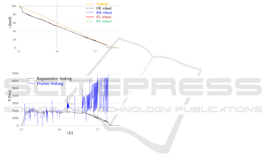
In Fig. 11, the braking diagrams obtained in

(Aksjonov et al., 2018) and confirmed experimentally

in (Aksjonov et al., 2019) are shown. They

demonstrate the velocities of the front left (FL), front

right (FR), rear left (RL), and rear right (RR) wheels,

appropriately, that follow the vehicle longitudinal

velocity in Fig. 11-(a), and EB and FB wheel torque

curves in Fig. 11-(b). Since the EB torque is not

sufficient to retain optimal slip, the control system

requests additional FB torque. At the end of slowing

down, regeneration turns off, and the FB completes

braking alone.

(a)

(b)

Figure 11: Experimental braking diagrams: (a) vehicle and

wheel velocities; (b) torque.

An original method was proposed in (Aksjonov et

al., 2018) for determining the road surface. Every

second, starting from ABS activation, the controller

evaluates the maximal deceleration of the vehicle and

compares it with the deceleration peaks preliminary

calculated using Eq. (8) at F

air

= β = 0. Such

momentary friction reset does not affect driving

comfort, as the process is very rapid, but it indicates

whether the road surface changes or remains the same

as before.

Alongside the set of positive outcomes, the

neglect of air friction, road slope, and other tire

features are the drawbacks of the above method. As

well, an evident chattering phenomenon at low

velocity is seen in the torque plots. In fact, its

appearance can be explained by three interrelated

reasons. First, this is an increase in static friction in

Eq. (5), when the vehicle is moving slowly and

several wheels tends to slip. Second, this is due to

high sensitivity of the slip to the velocity at slow

motion. Third, since at low velocity the EB ceases and

the FB finalises braking alone, there is no torque

stabilisation at that moment.

Torque oscillations demonstrate that the

simplified drive model used could not ensure proper

torque adjustment. Such kind of oscillation, reported

also by other researchers (Habibi and Yazdizadeh,

2010; Lin and Song, 2011; Li et al., 2018) is a

common issue of braking, needed to be considered as

it affects vehicle steerability and reduces energy

recovery.

9 COMPARING SIMULATIONS

TO EXPERIMENTAL RESULTS

The torque gradient approach proposed in the current

research brings sensitive benefits in braking

performance. Now, thanks to the close loop torque

control, there is no longer need to collect theoretical

tire-road friction data and determine the road surface.

Appropriate simulation diagrams plotted for the same

braking conditions as in (Aksjonov et al., 2019)

confirm these advantages. Since the optimal wheel

slip is approximately the same for both the front and

the rear left and right wheels, a quarter-vehicle model

described by Eqs. (1) – (6) is studied further.

Figure 12 introduces the traces obtained from the

friction-slip gradient control simulation. Here, the

total application torque (T, green) needed to ensure

intensive stopping in response to the driver’s setpoint

= 270 Nm is obtained after allocation between the

electric (T

, purple) and friction (T

, violet) torques,

wherein the electric torque is restricted to 200 Nm.

Since the motor response is much faster than that of

the friction unit, T

can be considered almost the same

as the demanded T

unless it exceeds the limitation

of the maximal electric power. Torque oscillations are

not observed here as they are damped by the torque

loop. At low velocity v

home

= 10 km/h, the friction

increases sharply due to its static fraction. The EB

turns off, and the torque begins fluctuate intensely.

Figure 13 confirms the effectiveness of the

torque-slip gradient control. Despite the fact that the

braking process lasts here 10% longer due to the

application torque delay and instability, the traces

look very similar to Fig. 12.

Fuzzy Gradient Control of Electric Vehicles at Blended Braking with Volatile Driving Conditions

257

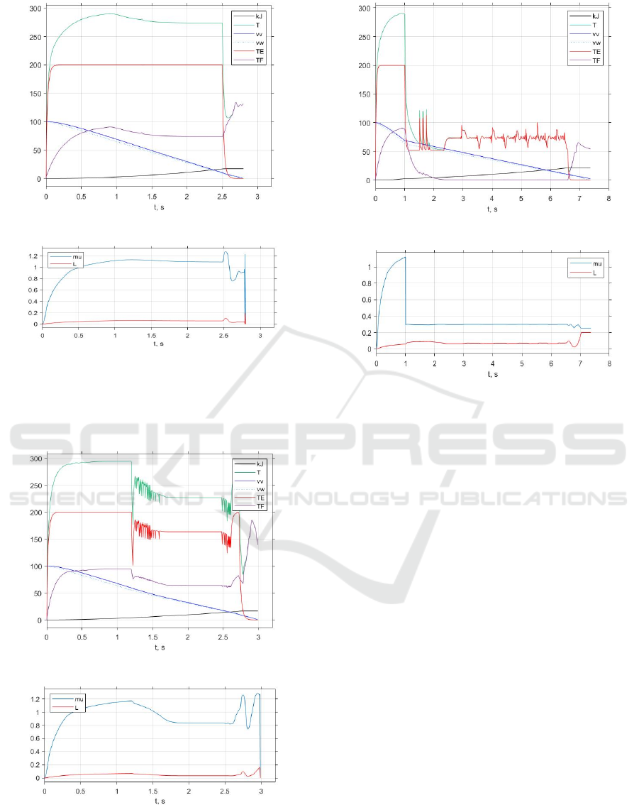
(a)

(b)

Figure 12: Friction-slip gradient braking diagrams at

constant tire-road friction: (a) – vehicle and wheel

velocities, electric, friction, and application torque, and

regenerative energy; (b) – tire-road friction and wheel slip.

(a)

(b)

Figure 13: Torque-slip gradient braking diagrams at

constant tire-road friction: (a) – vehicle and wheel

velocities, electric, friction and application torque, and

regenerative energy; (b) – tire-road friction and wheel slip.

(a)

(b)

Figure 14: Friction-slip gradient braking diagrams at

changing tire-road friction: (a) – vehicle and wheel

velocities, electric, friction, and application torque, and

regenerative energy; (b) – tire-road friction and wheel slip.

In order to investigate the effectiveness of the

proposed method in tracking more sophisticated

commands, vehicle motion above the changing road

surface was simulated. Figure 14 demonstrates the

traces obtained from the simulation of the volatile

driving using the friction-slip gradient control. Here,

the system successfully detects a change in road

conditions based on analysis of the friction-slip

gradient. At the beginning, the deceleration was

around 20 m/s

on a dry surface. At the end of the first

second, the road surface suddenly changes from dry

to wet. As the new gradient is recognized, the total

application torque needed to ensure an intensive stop

drops to 70 Nm. The FB is no longer requested

because the electric torque is sufficient to decelerate

the vehicle within the optimal wheel slip area.

Therefore, only electric braking is produced further.

However, when the speed drops below v

home

, the EB

turns off, friction braking resumes and the FB

operates alone.

Finally, Fig. 15 confirms the effectiveness of the

torque-slip gradient control at the volatile driving. It

represents the similar processes that take about 10%

longer braking time.

ICINCO 2020 - 17th International Conference on Informatics in Control, Automation and Robotics

258

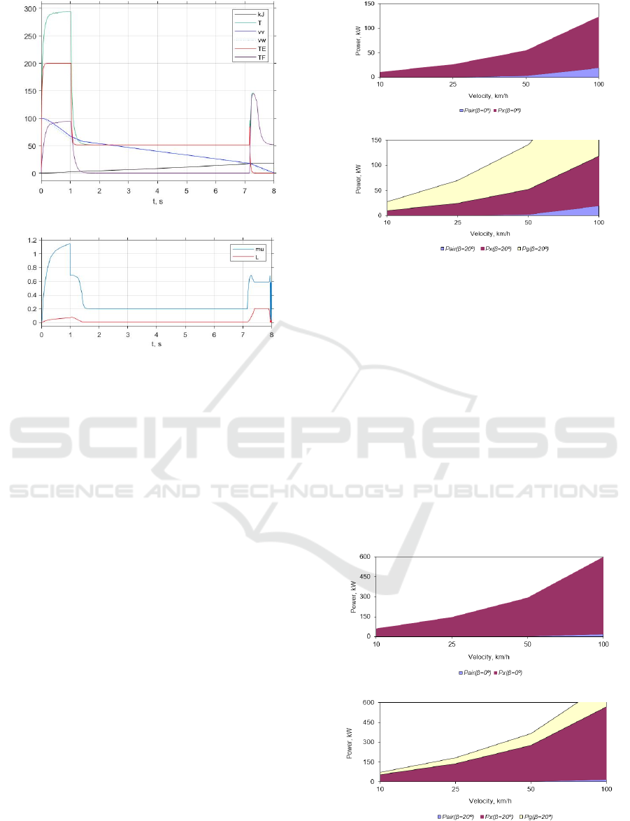
(a)

(b)

Figure 15: Torque-slip gradient braking diagrams at

changing tire-road friction: (a) – vehicle and wheel

velocities, electric, friction, and application torque, and

regenerative energy; (b) – tire-road friction and wheel slip.

Herewith, there is no more chattering in the torque

plots at low velocity. First, this is because the Wheel

block takes into account an increase of friction due to

its static fraction. Second, because the air friction is

involved in a close torque loop. Third and finally,

because the torque loop remains closed even without

the EB.

10 ANALYSIS OF ENERGY

RECOVERY

Based on the energy curves (kJ, black) and assuming

a 50% regenerative efficiency in Eq. (13), it turns out

from Figs. 12-(a) and 13-(a) that nearly 22 kJ of

energy is recovered during braking on the dry road.

In Figs. 14-(a) and 15-(a), despite the fact that the

stopping time is slightly increased, approximately the

same amount of energy is recovered as before.

To assess the degree of involvement of

aerodynamic and climbing resistances in energy

consumption and saving, simulation were performed

on the flat and 20º-downhill roads with different

velocities. An electric car with Q = 3 m

, ρ =

1.2 kg/m

, and C

air

= 0.5 was studied in the modes of

gradual (μ = 0.18) and intensive (μ = 1) braking.

(a)

(b)

Figure 16: Power components at gradual braking,  = 0.18:

(a) β = 0; (b) β = 20.

At gradual braking without inclination (β = 0 in

Fig. 16-(a)), the friction power (P

) dominates only at

low velocity, whereas in rapid cruising a significant

part of energy is spent on overcoming the air

resistance (P

air

). On the slope (β = 20 in Fig. 16-(b)),

much recovered energy can be released due to the

climbing counterforce (P

). At heavy braking, the

friction force (P

) always prevails on both the

longitudinal (Fig. 17-(a)) and inclined (Fig. 17-(b))

driveways. However, until the friction factor reaches

its upper level, it passes all intermediate levels, from

0.18 to 1, and all velocities, from v

to 0. This means

that both the volatile vehicle velocity and variable

friction must be taken into account in braking control.

(a)

(b)

Figure 17: Power components at heavy braking,  = 1:

(a) β = 0; (b) β = 20.

Fuzzy Gradient Control of Electric Vehicles at Blended Braking with Volatile Driving Conditions

259

11 CONCLUSION

In the refined vehicle model, multiple factors are

addressed, such as air resistance, road slope, and

changeable friction. An improved motor and energy

source model reflects the state of charge and electric

current/voltage restrictions of the hybrid energy

storage under various driving scenarios recognised by

the tire-road model, such as gradual deceleration and

emergency antilock braking in volatile driving

conditions. As a result, a proposed novel control

arrangement provides fuzzy adjustment and

stabilisation of the braking torque with a gradient

torque allocation between electric and friction brakes,

which allows integrating the advantages of both

friction and electric braking. Obtained simulation

diagrams largely coincide with the experimental

curves. They demonstrate consistently high braking

quality regardless of changes in the road surface and

slope, vehicle initial velocity, and air resistance.

ACKNOWLEDGEMENT

This work was supported by the Estonian Research

Council grant PRG658.

REFERENCES

Aksjonov, A., Vodovozov, V., Augsburg, K. and

Petlenkov, E., 2018. Design of regenerative anti-lock

braking system controller for 4 in-wheel-motor drive

electric vehicle with road surface estimation.

International Journal of Automotive Technology,

19(4):727 − 742.

Aksjonov, A., Vodovozov, V., Augsburg, K. and

Petlenkov, E., 2019. Blended antilock braking system

control method for all-wheel drive electric sport utility

vehicle. In ELECTRIMACS’19, 13th International

Conference of the IMACS TC1 Committee, Salerno,

Italy, pages 1 − 6.

Cecotti, M., Larminie, J. and Azzopardi, B., 2012.

Estimation of slip ratio and road characteristics by

adding perturbation to the input torque. In ICVES’12,

IEEE International Conference on Vehicular

Electronics and Safety, Istanbul, Turkey, pages 31 – 36.

Cerdeira-Corujo, M., Costas, A., Delgado, E., Barreiro, A.

and Banos, A., 2016. Gain-scheduled wheel slip reset

control in automotive brake systems. In SPEEDAM’16,

International Symposium on Power Electronics,

Electrical Drives, Automation and Motion, Anacapri,

Italy, pages 1255 – 1260.

Chen, Z., Lv, T., Guo, N., Shen, J., Xiao, R., Lu, X. and

Yu, Z., 2017. Study on braking energy recovery

efficiency of electric vehicles equipped with super

capacitor. In CAC’17, Chinese Automation Congress,

Jinan, China, pages 7231 – 7236.

Givigi Jr, S. N., Schwartz, H. M. and Lu, X. 2010. A

reinforcement learning adaptive fuzzy controller for

differential games. Journal of Intelligent and Robotic

Systems, 59(1):3 – 30.

Habibi, M. and Yazdizadeh, A., 2010. A novel fuzzy-

sliding mode controller for antilock braking system. In

2nd International Conference on Advanced Computer

Control, Shenyang, China, v. 4, pages 110 – 114.

Haidegger, T., Kovács, L., Preitl, S., Precup, R.-E.,

Benyó, B. and Benyó, Z. 2011. Controller design

solutions for long distance telesurgical applications.

International Journal of Artificial Intelligence, 6 (11

S):48 – 71.

Jing, H., Liu, Z. and Liu, J., 2011. Wheel slip control for

hybrid braking system of electric vehicle. In TMEE’11,

International Conference on Transportation,

Mechanical, and Electrical Engineering, Changchun,

China, pages 743 – 746.

Kadowaki, S., Ohishi, K., Hata, T., Iida, N., Takagi, M.,

Sano, T. and Yasukawa, S. 2007. Antislip adhesion

control based on speed sensorless vector control and

disturbance observer for electric commuter train AT

series 205-5000 of the east Japan railway company.

IEEE Transactions on Industrial Electronics,

54(4):2001 – 2008.

Kiyakli, O. and Solmaz, H., 2018. Modeling of an electric

vehicle with MATLAB/Simulink. International

Journal of Automotive Science and Technology,

2(4):9 – 15.

Li, W., Zhu, X. and Ju, J., 2018. Hierarchical braking torque

control of in-wheel-motor-driven electric vehicles over

CAN. IEEE Access, 6, pages 65189 – 65198.

Lin, H. and Song, C., 2011. Design of a fuzzy logic

controller for ABS of electric vehicle based on

AMESim and Simulink. In TMEE’11, International

Conference on Transportation, Mechanical, and

Electrical Engineering, Changchun, China, pages 779

– 782.

Naseri, F., Farjah, E. and Ghanbari, T., 2017. An efficient

regenerative braking system based on battery /

supercapacitor for electric, hybrid, and plug-in hybrid

electric vehicles with BLDC motor. IEEE Transactions

on Vehicular Technology, 66(5):3724 – 3738.

Pacejka, H., 2012. Tyre and Vehicle Dynamics (3rd ed.),

Oxford, UK: Butterworth–Heinemann.

Pratap, R. and Ruina, A., 2002. Introduction to Statics and

Dynamics. Oxford University Press.

Precup, R.-E., Tomescu, M.-L. and Dragos, C.-A. 2014.

Stabilization of Rössler chaotic dynamical system using

fuzzy logic control algorithm. International Journal of

General Systems, 43(5):413 – 433.

Radgolchin, M. and Moeenfard, H. 2018. Development of

a multi-level adaptive fuzzy controller for beyond pull-

in stabilization of electrostatically actuated microplates.

Journal of Vibration and Control. 24(5):860 – 878.

Reif, K. (Ed.), 2014. Brakes, Brake Control and Driver

Assistance Systems: Function, Regulation and

Components. Friedrichshafen, Germany: Springer.

ICINCO 2020 - 17th International Conference on Informatics in Control, Automation and Robotics

260

Savaresi, S. M. and Tanelli, M., 2010. Active Braking

Control Systems Design for Vehicles. London:

Springer.

Shang, M., Chu, L., Guo, J., and Fang, Y., 2010. Hydraulic

braking force compensation control for hybrid electric

vehicles. In CMCE’10, International Conference on

Computer, Mechatronics, Control and Electronic

Engineering, Changchun, China, pages 335 – 339.

Spichartz, P., Bokker, T. and Sourkounis, C., 2017.

Comparison of electric vehicles with single drive and

four wheel drive system concerning regenerative

braking. In EVER’17, 12th International Conference on

Ecological Vehicles and Renewable Energies, Monte-

Carlo, Monaco, pages 1 – 7.

Tao, Y., Xie, X., Zhao, H., Xu, W. and Chen, H., 2017. A

regenerative braking system for electric vehicle with

four in-wheel motors based on fuzzy control. In 36th

Chinese Control Conference, Dalian, China,

pages 4288 – 4293.

Xie, Y-B. and Wang, S-C, 2018. Research on regenerative

braking control strategy and Simulink simulation for

4WD electric vehicle. In ICMT’18, 2nd International

Conference on Manufacturing Technologies, Florence,

USA, pages 1 – 6.

Xu, W., Zhao, H., Ren, B. and Chen, H., 2016. A

regenerative braking control strategy for electric

vehicle with four in-wheel motors. In 35th Chinese

Control Conference, Chengdu, China, pages.

8671 – 8676.

Zhang, X. and Lin, H., 2018. UAV anti-skid braking system

simulation. In 37th Chinese Control Conference,

Wuhan, China, pages 8453 – 8458.

Fuzzy Gradient Control of Electric Vehicles at Blended Braking with Volatile Driving Conditions

261