Consistency Analysis of AUTOSAR Timing Requirements

Steffen Beringer

1 a

and Heike Wehrheim

2 b

dSPACE GmbH, Rathenaustr. 26, 33102 Paderborn, Germany

Department Speciﬁcation and Modelling of Software Systems, Paderborn University, 33102 Paderborn, Germany

Keywords:

AUTOSAR, Consistency Analysis, Timing Analysis, Timing Constraints, Satisﬁablilty Modulo Theories,

Maximum Satisﬁability, Unsatisﬁable Core, Timed Automata.

Abstract:

Applying formal methods in the automotive industries can signiﬁcantly increase the correctness and reliability

of the developed system architectures. This in particular demands a formal speciﬁcation and analysis of

requirements on systems. Automotive software architectures are, however, often described using the (semi-

formal) AUTOSAR standard which is based on various meta models as exchange formats. This complicates

a formal analysis. In this paper, we provide a formalization of timing requirements within the AUTOSAR

standard. Timing requirements specify constraints on events of the underlying software architecture. We

provide a translation of timing requirements into logical constraints which enable the usage of SMT solvers to

analyse requirements. Speciﬁcally, we employ this translation to check consistency of the requirements and

use maximum satisﬁability solving for localization of erroneous requirements.

1 INTRODUCTION

For the distributed development of various automotive

software, the automotive industry utilizes the features

of the de facto standard AUTOSAR (AUTOSAR,

2019). It provides a common infrastructure for auto-

motive systems of all vehicle domains based on stan-

dardized interfaces. This also includes the deﬁnition

of component-based software architectures. It further

comprises a methodology how to facilitate and paral-

lelize the development of AUTOSAR architectures.

AUTOSAR provides methods for specifying tim-

ing requirements on the underlying software archi-

tecture by the so called AUTOSAR timing constraints

meta-model extension. Different types and ﬂavors of

timing constraints allow for an easy use for different

parts of the software architecture in different develop-

ment phases.

Nevertheless, when the requirements get numer-

ous, maintaining an overview of them can be hard and

hence inconsistencies in the requirements can occur.

Inconsistent requirements are an indication for a mis-

understanding of the expected system functionality by

the software developer. Moreover, when requirements

are formally checked against the system architecture,

e.g. via timing veriﬁcation methods as described in

https://orcid.org/0000-0002-8504-7435

https://orcid.org/0000-0002-2385-7512

(Beringer and Wehrheim, 2016) or (Richter, 2005),

inconsistent requirements lead to unnecessary veriﬁ-

cation runs since veriﬁcation is then inevitably going

to fail for some of the requirements. It is advanta-

geous to know inconsistencies in the requirements be-

forehand.

act VerificationProcessActivityDiagram

Check Consistency (R) Compute R' = MaxSMT(R)

&& R'' = unsatcore(R)

Verify (M, R)

Revise R according to R'

and R''

[R UNSAT]

[R SAT]

Figure 1: Analysis process described as UML activity dia-

gram.

This work thus presents an approach for support-

ing the early validation of AUTOSAR software ar-

chitectures by simplifying the process of AUTOSAR

timing requirements speciﬁcation. It comprises an

analysis method which checks a deﬁned set of AU-

TOSAR timing requirements for inconsistencies by

transformation of requirements models into satisﬁ-

able modulo theories (SMT) formulae. This enables

checking requirements before any further veriﬁca-

tion task is triggered and assists a requirements en-

gineer in ﬁxing the requirements set. Furthermore, it

supports the identiﬁcation of possible inconsistency

Beringer, S. and Wehrheim, H.

Consistency Analysis of AUTOSAR Timing Requirements.

DOI: 10.5220/0009766600150026

In Proceedings of the 15th International Conference on Software Technologies (ICSOFT 2020), pages 15-26

ISBN: 978-989-758-443-5

causes. Whenever the set of SMT formulae is unsat-

isﬁable (and hence the requirements inconsistent), we

compute the maximal subset of satisﬁable formulae

(MaxSMT). These represent a set of consistent re-

quirements. All requirements which are not in this

set are potential inconsistency causes. By further-

more computing an unsatisﬁable core of formulae,

we narrow down the requirements to look at for in-

consistency resolution. A visualization of both unsat

core and MaxSMT result helps the requirements en-

gineer in ﬁxing errors. Note that we do not run the

requirements check on any transformed veriﬁcation

model (e.g. timed automata when checking the re-

quirements as described in (Beringer and Wehrheim,

2016)), but directly on the AUTOSAR timing con-

straints model. This approach is advantageous, since

it decouples the concistency check from the speciﬁc

veriﬁcation method.

An overview of the proposed steps and their exe-

cution sequence is shown in Figure 1 and comprises

the following ﬁve steps (for a given set of require-

ments R and given architecture model M):

1. Check the consistency of requirements R .

2. If the complete set is not consistent, compute the

greatest subset of veriﬁable constraints R

(via

a maximum satisﬁability solver) and R

a min-

imum subset of constraints, which is inconsistent,

otherwise go to step 5.

3. Revise the requirements R based on the informa-

tion by R

and R

4. Repeat steps 1-3 until the requirements are con-

sistent.

5. Perform veriﬁcation process on the requirements

set and the architecture model (M, R ).

All steps within the analysis process are fully au-

tomated and implemented prototypically for the

dSPACE AUTOSAR authoring tool SystemDesk

1

For step 5, we transform the given AUTOSAR archi-

tecture model into timed automata and the require-

ments into test automata and timed computational

tree logic queries (TCTL). The approach for this has

been proposed in (Beringer and Wehrheim, 2016).

Note that steps 1-4 are performed on the requirements

model only. The architecture model is used in step 5.

The paper is organized as follows. The next sec-

tion 2 introduces the domain of AUTOSAR, the con-

cept of timing requirements, and introduces a ﬁrst ex-

ample model. Transformation of requirements into

SMT-formulae and our approach for identiﬁcation

and correction of inconsistent requirements are shown

http://www.dspace.com/en/pub/home/products/sw/

\system architecture software/systemdesk.cfm

in Sections 3 and 4, respectively. Thereafter, runtime

measurement results for requirements transformation

and veriﬁcation are presented in Section 5. Finally,

Section 6 discusses existing work related to our ap-

proach following a conclusion in Section 7, which

summarizes the achievements in this work and give

hints for future improvements.

2 BACKGROUND

In this chapter we introduce the foundations of AU-

TOSAR and the AUTOSAR timing extensions used to

specify timing requirements. We brieﬂy discuss con-

sistency in general and introduce our running example

model.

2.1 AUTOSAR

AUTOSAR

is short for AUTomotive Open System

ARchitecture and is a joint standard developed by var-

ious automobile manufacturers, suppliers, tool ven-

dors, services- and semiconductor companies. AU-

TOSAR deﬁnes the architecture and interfaces of

software as meta-model as well as the ﬁle format for

data exchange. Furthermore, the standard deﬁnes its

own development methodology. The concepts of this

work are based on the current AUTOSAR release ver-

sion 4.3.

AUTOSAR Software Architecture. On the high-

est level AUTOSAR deﬁnes a layered software ar-

chitecture, which contains three layers (AUTOSAR,

2019). The application layer contains the controller

software and is structured as component-based archi-

tecture, which means software components can be de-

ﬁned, which communicate via ports. Components

contain one or more so-called runnable entities (or

runnables in short) Re = {re

, .. . , re

}, which con-

tain executable software. The runtime environment

layer provides standardized APIs to connect the com-

ponents and modules on the basic software layer,

whereas the basic software layer provides modules

for basic ECU functions like the operating system and

communication services and is again subdivided into

layers (see e.g. Figure 2).

AUTOSAR Timing Extensions. A subset of the

AUTOSAR meta-model addresses the annotation of

model elements with timing properties (AUTOSAR,

2019). For a set of model elements so-called timing

events E = {e

. . . e

} can be speciﬁed. A timing event

http://www.autosar.org

ICSOFT 2020 - 15th International Conference on Software Technologies

is the abstract representation of a speciﬁc system be-

havior that can be observed at runtime, e.g. the start of

a runnable or the arrival of new data at a port. Further-

more, AUTOSAR timing extensions enable the deﬁ-

nition of timing constraints R = {r

, . . . , r

}, which

deﬁne a timing relationship between two or more tim-

ing events. Timing constraints can be deﬁned by re-

stricting the execution times of runnable entities. The

following timing constraints are considered:

Offset Timing Constraint. An offset timing con-

straint r

otc

= (e

, e

, min, max) constrains the time

between a source timing event e

∈ E and tar-

get timing event e

∈ E by deﬁning a minimum

and maximum offset min,max ∈ R between those

events.

Latency Timing Constraint. A latency timing con-

straint r

ltc

= (C, min, max) describes a minimum

and maximum latency in the scope of a timing

chain C. The timing chain is an ordered sequence

of events, C = he

, . . . , e

i, e

∈ E for all 1 ≤ i ≤ n,

which have to occur in the speciﬁed time bound.

Synchronization Timing Constraint. A syn-

chronization timing constraint r

stc

(S, tolerance), S ⊆ E speciﬁes a set of tim-

ing events, which must occur simultaneously

within a tolerance value.

Execution Order Constraint. An execution order

constraint r

eoc

= hre

, . . . , re

i constrains the ex-

ecution order of runnable entities. So for each

execution order constraint r

eoc

∈ R

eoc

with an or-

dered set of runnable entities hre

. . . re

i a suc-

cessor runnable entity re

i+1

may only be executed

after the runnable entity re

has been executed.

Execution Time Constraint. The execution time

constraint r

etc

= (re, min, max) does not restrict

the occurrence of timing events, but the execution

time of an executable entity re to a minimum

duration min and maximum duration max. The

runnable re can be either a runnable entity on the

application layer or a basic software module on

the basic software layer.

A software developer can deﬁne a number of such re-

quirements on a given AUTOSAR software architec-

ture. Further timing constraints like Age Timing Con-

straint are not considered since they do not add in-

consistencies in our approach, because they only ref-

erence one timing event and restrict the timing of a

variable implicitly. For modeling of AUTOSAR tim-

ing constraints we employ SystemDesk



The AUTOSAR Authoring Tool SystemDesk.

SystemDesk



is the tooling environment for AU-

TOSAR models of the company dSPACE. It supports

sophisticated and extensive modeling of AUTOSAR

architectures by providing a rich graphical user in-

terface as well as code generation for virtual ECUs.

Graphical model representations are available for im-

portant elements. For example, software components,

ports and connections within a software composition

can be visualized in a composition diagram. Further-

more, single software components with their ports,

interfaces and data types can be visualized in a com-

ponent diagram. Other model elements are ordered

hierarchically in a tree structure.

2.2 Consistency of Requirements

Our interest here is in checking consistency of such

timing requirements. The IEEE recommendations

for software requirements speciﬁcations (IEEE, 1998)

calls a software requirements set consistent ”if, and

only if, no subset of individual requirements de-

scribed in it conﬂict”. This means that the set of

requirements is consistent, if there exists a model or

system, which can satisfy all requirements in this set.

Deﬁnition 1 (Consistency). Let R = {r

, . . . , r

} be

the set of timing requirements in an AUTOSAR model

and let M be the set of models. Then R is consistent

iff ∃M ∈ M : ∀r

∈ R : M |= r

In the case of AUTOSAR the set of models is de-

ﬁned by all models which can be modeled using the

AUTOSAR meta-model and the requirements are de-

ﬁned by a set of AUTOSAR timing constraints. Thus,

the set of AUTOSAR timing constraints is only con-

sistent, if there is a AUTOSAR model which con-

forms to all restrictions imposed by the AUTOSAR

timing constraints. Since the timing constraints re-

strict the model’s behavior only in the sense of tim-

ing, the only model elements of interest are the AU-

TOSAR timing events. Therefore, checking the ex-

istence of a valid model is reduced to ﬁnding a valid

execution order of timing events.

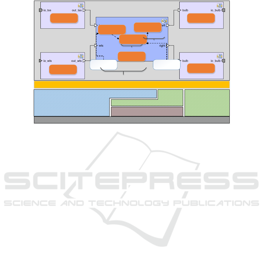
2.3 AUTOSAR Example: The Turn

Switch Indicator

In the following we will consider a simple AUTOSAR

software architecture. The architecture manages left

and right direction indicators of a vehicle according to

turn switch and warn lights sensors. The application

layer consists of several software components which

comprise several so-called runnable entities contain-

ing executable software. The example architecture is

shown in Figure 2. The two software components on

the left read in sensor data and check for errors be-

fore forwarding the signal data to the next software

Consistency Analysis of AUTOSAR Timing Requirements

Application layer

Runtime environment

Microcontroller

TssRunnable

WlsRunnable

TurnSwitchSensor

WarnLightsSensor

FrontLeftActuator

FrontRightActuator

TssPre-

processing

WlsPre-

processing

Logic

Toggle

IndicatorComposition

BulbRunnable

Complex Drivers

Microcontroller Abstraction Layer

ECU Abstraction Layer

Services Layer

e_s_TssPre-

processing

e_t_Logic

10|30

3|4

1|5

Figure 2: Example Software Architecture.

component. The Indicator Composition software

component receives the raw sensor values and encap-

sulates several runnable entities for pre-processing of

the signal values as well as the logic of the system.

The actuator software components on the right are

responsible for activating the left respectively right

bulb of the direction indicator. Furthermore, the ex-

ample contains a conﬁguration of the RTE, and on

the basic software layer the conﬁguration for the op-

erating system. Other basic software modules are

not considered in this example. Furthermore, the

example is extended with the following timing de-

scription events and timing constraints. The runnable

TssPreprocessing consists of an event for the start

TssPreprocessing

, and for runnable Logic an event for

its termination e

Logic

has been added. These timing

events are shown as white boxes in the example di-

agram, connected to the runnable entity they belong

to. Additionally, the architecture contains three tim-

ing constraints: An execution order constraint con-

straining the execution of runnable entities, which

is shown as dashed lines between runnables; an off-

set timing constraint constraining the time between

newly added timing events, which is reﬂected by the

brackets among the timing events, and an execution

time constraint constraining the execution time of the

Logic runnable (see also Table 1).

This set of constraints is not consistent. The

Logic runnable must take at least 10ms for execution

etc

), while the calculation of the indicator logic shall

be completed between 3ms and 4ms after the turn

switch sensor pre-processing has been started (r

otc

This includes the computation of the Logic runnable,

since the runnables TssPreprocessing and Logic

must be executed in order (because of r

eoc

). Our

approach automatically identiﬁes this kind of incon-

sistencies, while a manual inspection would be quite

complex since the inconsistency results from different

types of timing constraints. We consciously stick to

only three different constraints in our example to keep

it comprehensible, although we implemented our ap-

proach for all of the presented timing constraints.

3 TRANSFORMATION OF

AUTOSAR TIMING

CONSTRAINTS

For consistency checking of timing requirements, we

use a logical approach. In this section we describe the

transformation of AUTOSAR timing requirements

into logical formulae of an SMT (satiﬁability modulo

theories) solver. The SMT formulae reﬂect the tempo-

ral constraints predeﬁned by the timing requirements

and thus satisﬁability conforms to the existence of a

valid ordering of timing events satisfying all require-

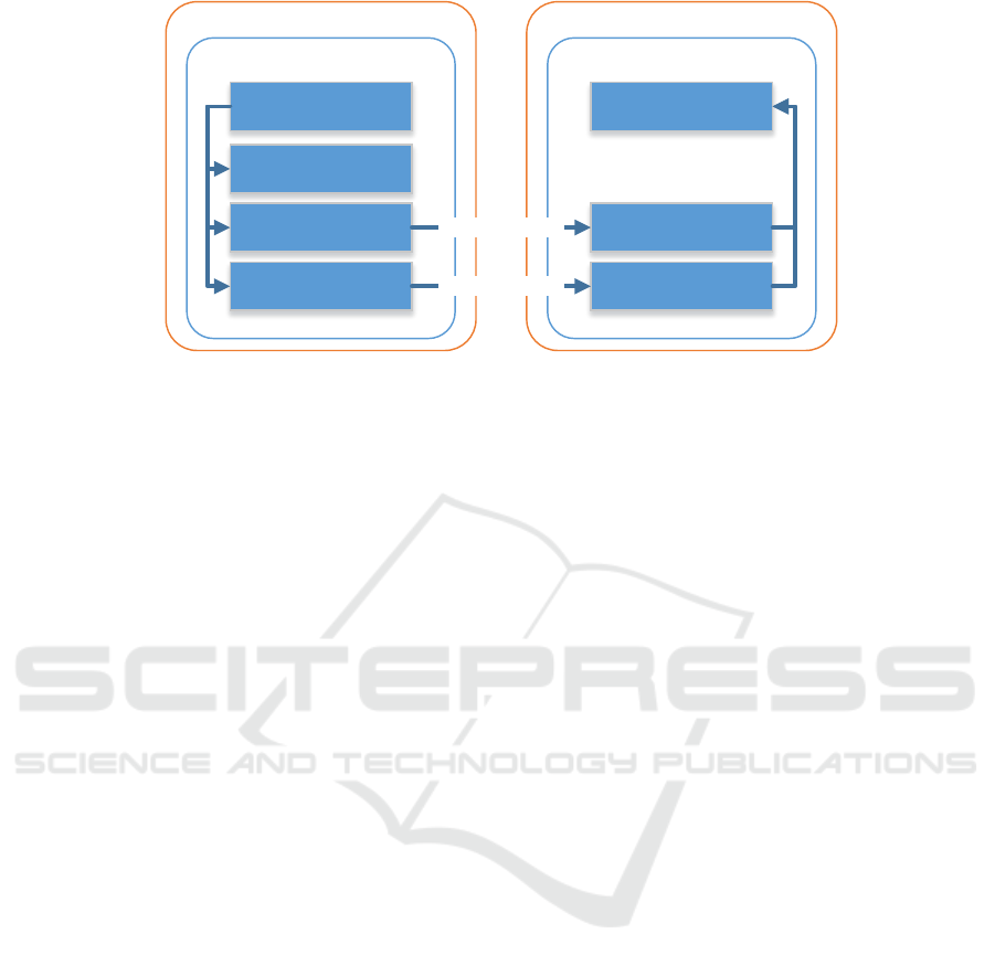
ments. In Figure 3 the abstract concept is shown. The

AUTOSAR model contains the system model, tim-

ing events, which are associated to model elements

in the system model and the AUTOSAR timing con-

straints. The timing events are transformed into SMT

variables and the AUTOSAR timing events are trans-

formed into linear constraints over the generated vari-

ables, while the system model is not needed for the

consistency analysis. The transformations have been

ICSOFT 2020 - 15th International Conference on Software Technologies

Table 1: Example Timing Constraints.

Description Requirement

The runnable entities

TssPreprocessing, Logic and

Toggle must be executed in order.

eoc

= hTssPreprocessing, Logic, Togglei

The calculation of the indicator

logic shall be completed between

3ms and 4ms after the turn switch

sensor preprocessing has been

started.

otc

= (e

TssPreprocessing

, e

Logic

, 3, 4)

The calculation of the Logic

runnable should be completed in

between 10ms and 30ms.

etc

= (Logic, 10, 30)

The calculation of the Toggle

runnable should be completed in

between 1ms and 5ms.

etc

= (Toggle, 1, 5)

automated and are directly applied on the AUTOSAR

model within SystemDesk.

Some timing constraints are not only based on

timing events, but on runnable entities, for exam-

ple the execution order constraint. To detect incon-

sistencies between those timing constraints and tim-

ing constraints based on timing events, timing con-

straints based on runnable entities are transformed so

that they are also based on timing events. This is

possible since AUTOSAR supports timing events re-

lated to the execution of runnable entities. Thus in

the following we assume that for each runnable en-

tity re ∈ RunnableEntities there exist corresponding

timing events e

and e

, which represent the exe-

cution start and termination of the runnable entity.

Some timing constraints also restrict the occurrence

between timing events, thus lower and upper bounds

itself can be deﬁned by the occurrence of another tim-

ing event. Nevertheless, all restrictions can be deﬁned

as linear constraints. Since the restrictions on tim-

ing events are deﬁned by linear constraints, the ex-

istence of a valid model can be checked by search-

ing for a valid valuation t : E → R

≥0

of the tim-

ing events using a SMT solver with linear arithmetic.

For this, we use the SMT solver Z3 (Bjorner and

Phan, 2014). For a given AUTOSAR model with

timing events E = {e

. . . e

} and timing constraints

R = (r

, . . . , r

) an SMT formula F =

i=1

is suc-

cessively constructed. Each term in F is either a con-

stant constraint value (e.g. tolerance or minimum /

maximum values) or a variable, which conforms to a

timing event e and which needs a satisfying assign-

ment into the time domain t : E → R

≥0

. We de-

note the sets of different timing constraint types as

R = R

otc

∪ R

ltc

∪ R

stc

∪ R

eoc

∪ R

etc

. In the following

the transformation for each type of timing constraint

is presented.

Offset Timing Constraint. An offset timing con-

straint r

otc

= (e

, e

, min, max) constrains the time be-

tween a source timing event e

and target timing event

. Thus, for each timing offset constraint r

otc

∈ R

otc

two expressions are added to the SMT formula as fol-

lows

otc

= e

+ max ≥ e

∧ e

+ min ≤ e

(1)

Latency Timing Constraint. To verify that a la-

tency timing constraint does not conﬂict with other

timing constraints, for example an offset timing con-

straint, there must be a valid occurrence of timing

events where there exists a sequence of timing events,

which does not exceed the maximum value of a la-

tency timing constraint. Therefore, for each ltc with

chain C = he

, . . . , e

i the SMT formula is extended

as follows

ltc

= ∀i, 1 ≤ i ≤ n − 1 : e

≤ e

i+1

∧min ≤ e

− e

≤ max

(2)

Synchronization Timing Constraint. A synchro-

nization timing constraint r

stc

= (S, tolerance), S ⊆ E,

speciﬁes a set of timing events, which must occur si-

multaneously with a tolerance value. So for each syn-

Consistency Analysis of AUTOSAR Timing Requirements

Z3SystemDesk

Specification Model Analysis Model

AUTOSAR Model

Timing Events

AUTOSAR

Timing Constraints

Variables

Linear Constraints

SMT Formulae

<<transforms to>>

AUTOSAR

System Model

Figure 3: Transformation of AUTOSAR models into SMT formulae.

chronization timing constraint r

stc

∈ R

stc

, the toler-

ance value is checked for each combination of events:

stc

= ∀e, e

∈ S : e − e

≤ tolerance (3)

Execution Order Constraint. For each execution or-

der constraint r

eoc

∈ R

eoc

with a sequence of runnable

entities hre

, . . . , re

i a successor runnable entity re

i+1

may only be executed after the runnable entity re

has

been executed. Thus, ∀i, 1 ≤ i < n : re

≤ re

i+1

. Since

our approach relies on ﬁnding a satisﬁable assignment

based on timing events, we ﬁrst need to ﬁnd a mod-

eling alternative, which is equivalent, but is based on

timing events instead of runnable entities. Therefore,

we model the constrained execution of runnable en-

tities by timing events, which represent the start and

stop of a deﬁned runnable and only allow the start

event of a succeeding runnable entity to be later than

the termination event of the runnable entity before. So

let e

and e

be the start and terminated event of a

runnable re

. Thus we get

∀i, 1 ≤ i ≤ n − 1 : e

≤ e

∧ e

≤ e

i+1

(4)

AUTOSAR also allows execution order constraint to

be applied to basic software modules. The naming of

timing events then is different, but the general trans-

formation method presented can be applied analo-

gously.

Execution Time Constraint. The restriction in an

execution time constraint is only within a single AU-

TOSAR element. Nevertheless, a restriction of the

execution time corresponds to having a offset tim-

ing constraint between the execution start and termi-

nation of the associated runnable. Therefore, a exe-

cution time constraint corresponds to having an off-

set timing constraint r

etc

= (r, min, max) = r

otc

with

otc

= (e

, e

, min, max) where e

and e

are the

events associated with the runnable being started and

terminated, respectively.

The generated SMT formulae for the example model

are shown in Table 2. For the execution order con-

straint r

eoc

start events for each runnable must oc-

cur before the corresponding termination event and

the start event for runnable Logic must be before the

termination event of runnable TssPreprocessing.

Analogously the termination event of runnable Logic

must occure before the start event for the Toggle

runnable occurs. Therefore, our approach generates

ﬁve inequalities, which constrain the timings as de-

scribed. For the Offset Timing Constraint r

otc

two

inequality clauses are generated, which constrain the

minimum and maximum offset for the timing events.

Finally, for the execution time constraints r

etc

and

etc

two clauses are generated for each constraint,

which constrain the timing for the start and termina-

tion of the Logic runnable and the Toggle runnable

respectively. Since the requirements are not consis-

tent, the generated set of clauses is unsatisﬁable.

4 RESOLVING INCONSISTENT

REQUIREMENTS

In this section we describe methods to resolve incon-

sistent requirements. For this, we propose to compute

the maximum set of satisﬁable clauses as well as an

unsatisﬁable core and visualize the results.

4.1 Identiﬁcation of Inconsistency

Causes

To identify defects in an unsatisﬁable requirements

set we investigate several methods, which compute a

subset of timing requirements associated with consis-

tency. First we compute the maximum set of satisﬁ-

able clauses (MaxSMT) (Bjorner and Phan, 2014).

ICSOFT 2020 - 15th International Conference on Software Technologies

Table 2: Example Transformations.

Requirement Generated formulae

eoc

hTssPreprocessing, Logic, Togglei

= e

TssPreprocessing

≤ e

TssPreprocessing

= e

Logic

≤ e

Logic

= e

Toggle

≤ e

Toggle

= e

TssPreprocessing

≤ e

Logic

= e

Logic

≤ e

Toggle

otc

= (e

TssPreprocessing

, e

Logic

, 3, 4)

= e

TssPreprocessing

+ 3 ≤ e

Logic

= e

TssPreprocessing

+ 4 ≥ e

Logic

etc

= (Logic, 10, 30)

= e

Logic

+ 10 ≤ e

Logic

= e

Logic

+ 30 ≥ e

Logic

etc

= (Toggle, 1, 5)

= e

Toggle

+ 1 ≤ e

Toggle

= e

Toggle

+ 5 ≥ e

Toggle

Deﬁnition 2 (Weighted MaxSMT). Given a set of for-

mulae F and numeric weights w ∈ W associated with

each formula by a function c : F → W , the task of

weighted maximum satisﬁability solving modulo the-

ories (MaxSMT) is to ﬁnd a subset I ⊆ F such that

f ∈I

f is satisﬁable and

∑

f ∈I

c( f ) is maximal in all subsets of F .

Thus, if the set of requirements is not satisﬁable,

MaxSMT ﬁnds a subset of formulae which maximizes

a deﬁned cost function c. In our case, c( f ) = 1 for all

formulae f , so we give no priorities to certain con-

straints.

Applying MaxSMT in this case ﬁnds a largest set

of formulae which are satisﬁable. Furthermore, for

traceability we keep a mapping r : F → R , which

maps each formula f back to the timing require-

ment it originated from. With this information a re-

quirements engineer might ﬁx the requirements set

by either discarding or altering / relaxing require-

ments which do not belong to the MaxSMT set, so

that ﬁnally the complete requirements set is satisﬁ-

able. The MaxSMT computation is performed in Z3.

A MaxSMT subset for our example is I = R \ { f

Another method for identiﬁcation of inconsisten-

cies are unsatisﬁable cores (unsat core in short).

Deﬁnition 3. Let F be a set of formulae which is

unsatisﬁable. An unsatisﬁable core of F is a subset

F ⊆ F which is unsatisﬁable as well.

SMT solvers typically try to compute minimal un-

sat cores. However, neither unsat cores nor MaxSMT

solutions are unique. Given the MaxSMT solution,

and in particular a set of requirements R which are

not part of this solution (and thus potentially incor-

rect), we can compute an unsat core to get the set of

formulae (requirements) which are together inconsis-

tent. Ideally, this is not the entire set of requirements

so that the requirements engineer does not need to

look at all requirements when trying to identify and

correct wrong requirements.

In our example an unsat core would be UC =

{ f

, f

}. For those constraints there is no

satisﬁable ordering of the events e

TssPreprocessing

, e

Logic

and e

Logic

. Since r

etc

does

not contain any clauses of the unsat core, this require-

ment is not responsible for the inconsistency. Thus,

here we can use the unsat core to narrow down the set

of requirements to look at during correction.

4.2 Consistency Visualization

A crucial point for the identiﬁcation of inconsistency

causes is an adequate result visualization of the gen-

erated MaxSMT and unsat core clauses. In this re-

gard we provide a graph-based visualization of the

MaxSMT and unsat core, where nodes in the graph

represent timing events and directed edges represent

the timing relations (i.e., the SMT clauses) among the

events.

Deﬁnition 4 (ResultGraph). Given a set of timing

events E and the set of transformed requirement for-

mulae F , the result graph G = (G

, G

, c

min

, c

max

) is

the following:

• G

= E is the set of nodes containing one node

per timing event,

• G

⊆ G

× G

is the set of directed edges, where

(e, e

) ∈ G

if the set F contains a formula e ≤

Consistency Analysis of AUTOSAR Timing Requirements

or e + min ≤ e

or e + max ≥ e

for some

min, max ∈ R,

• c

min

: G

→ 2

is the minimum distance labeling

function, where min ∈ c

min

(e, e

) if the set F con-

tains a formula e + min ≤ e

• c

max

: G

→ 2

is the maximum distance label-

ing function, where max ∈ c

max

(e, e

) if the set F

contains a formula e + max ≥ e

For the MaxSMT and unsat core two result graphs

are visualized separately. In the MaxSMT result

graph G

max

nodes are labeled green, if the corre-

sponding clauses, which represent the timing rela-

tions among the events, belong to I and red otherwise.

For the unsat core result graph G

nodes are labelled

green, if they do not belong to UC and green other-

wise.

4.2.1 Example Visualization

Figure 4 shows the graphical representation of the

(generated) events and the timing relationships among

them utilizing our example transformations shown in

Table 2. Timing events which belong to satisﬁable

timing requirements are shown in green, while timing

events which belong to unsatisﬁable timing require-

ments are shown in red.

5 EVALUATION

In this section, we evaluate the runtime of our ap-

proach based on example architectures. We ﬁrst

evaluate the runtime of the requirements consistency

checking approach and try to ﬁgure out whether the

application to real-world projects is feasible. After-

wards we argue if and how the consistency check-

ing and our timing veriﬁcation approach can be ef-

ﬁciently combined and whether our proposed pro-

cess in Figure 1 is reasonable. Since the generated

SMT formulae are linear constraints and the consid-

ered domain is the set of rational numbers, the model

can be solved using the general simplex algorithm

and thus the model is solvable in polynomial runtime

(Kroening and Strichman, 2008). To identify pos-

sible defects in an unsatisﬁable requirements set we

compute the maximum set of satisﬁable constraints

(MaxSMT). Since the MaxSMT problem is NP-hard,

we presume higher runtime (Garey et al., 1976). Nev-

ertheless, MaxSMT comutation should still be faster

than the veriﬁcation task itself, because the trans-

formed timed automata model has exponential run-

time in the number of clocks, which can be rather

high, since the full AUTOSAR architecture is trans-

formed. For each test scenario we measure the time

for requirements transformation and the SMT solver

as well as the veriﬁcation time for the approach de-

scribed in (Beringer and Wehrheim, 2016).

5.1 Test Scenarios

First, the runtime for requirements transformation,

SMT solving and MaxSMT optimization is measured

for each timing constraint type separately and for a set

of different combined timing constraint types. With

this step we identify, if for a predeﬁned size of re-

quirements the runtime for consistency checking and

MaxSMT computation is reasonable. For the mea-

surement of SMT solving and requirements transfor-

mation the timing constraints were generated. For

an offset timing constraint a source and target tim-

ing event with a minimum and maximum offset be-

tween 1ms and 10ms were selected randomly. For an

execution order constraint 5 runnables were selected

randomly and for each synchronization timing con-

straint 3 timing events were selected randomly. We

limit the size to 10, because otherwise the timing ver-

iﬁcation task takes too long. For the MaxSMT opti-

mization measurement we generated an unsatisﬁable

set, for which the solver computes the maximum sat-

isﬁable set. Afterwards the runtime for timing veriﬁ-

cation is measured based on two different generated

architecture models and compared to the consistency

check to have an idea whether consistency checking

is generally favorable before the veriﬁcation task to

save time. One model M

contains only of a lim-

ited set of software components and very few tasks,

whereas a second model M

is more complex con-

taining more software components and tasks. Table 4

gives an overview of the complexity of those models.

Since most of the requirements sets generated are in-

consistent, the subsequent timing veriﬁcation would

fail for at least one requirement.

5.2 Evaluation Setup

The SMT solver used is Z3 version 4.6.0-x64. For

timing veriﬁcation UPPAAL version 4.0.13 is used

(Behrmann et al., 2004). The test scenario execution

and runtime measurement is performed on a Windows

7 Professional system with an Intel Core i7 4800MQ

with 8GB memory. UPPAAL was used with BFS

search order, conservative state space reduction and

DBM state space representation. The runtime is mea-

sured in seconds. The symbols used in the results are

explained in Table 3.

ICSOFT 2020 - 15th International Conference on Software Technologies

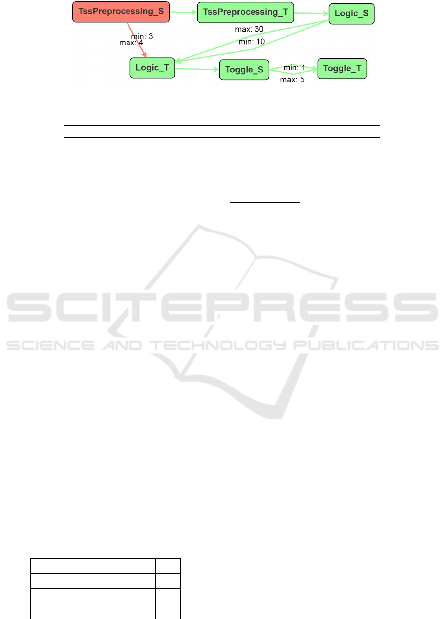
Figure 4: ResultGraph for MaxSMT.

Table 3: Description of symbols.

Symbol Description

T (t) Runtime for transformation of requirements into SMT in seconds

T (smt) Runtime for SMT solving in seconds

T (msat) Runtime for MaxSMT in seconds

T (tv) Runtime for model transformation into timed automata

T (v) Runtime for timing veriﬁcation in seconds

ratio Runtime ratio in percentage

T (t)+T (smt)+T (msat)

T (tv)+T (v)

∗ 100

5.3 Results

Table 5 shows runtime measurements for the compu-

tation of the maximum satisﬁable set of constraints

and the timing veriﬁcation for both M

and M

. The

table shows, that transformation of the AUTOSAR el-

ements into Z3-SMT takes a signiﬁcant amount of

time (T (t)). This is partly due the fact that the ele-

ments are accessed via an automation interface of the

AUTOSAR authoring tool, which is less efﬁcient than

a direct access due to technological reasons. Further-

more, the transformation algorithm has not been op-

timized by now. Nevertheless, the time is acceptable

compared to the time needed for timing veriﬁcation.

T(t), T(smt) and T(msat) are identical for test sce-

narios with the same requirements R , even on dif-

ferent architecture models (e.g. test scenarios 1 and

5). This is evident since the runtimes, which belong

to the requirements checking part, are independent of

the rest of the AUTOSAR architecture.

The model transformation into timed automata

and the veriﬁcation runtime is obviously largely de-

pendent on the size and complexity of the overall

AUTOSAR architecture model. While transformation

and veriﬁcation of the requirements of M

is fast with

a maximum runtime of 20.1 and 11 seconds for test

scenario 4, the same requirements embedded in ar-

Table 4: Test scenarios for veriﬁcation runtime.

Software Components 5 8

Runnable Entities 10 80

Tasks 5 8

chitecture M

can take up to roughly 2 minutes for

transformation and 36 minutes for veriﬁcation in test

scenario 8. Finally, we measured the runtimes for the

running example, which consists of 5 software com-

ponents, 8 runnables and 3 tasks, which is a rather

simple model. The transformation and consistency

check took 4.5 and 0.1 seconds respectively, while

veriﬁcation took only 1.4 seconds.

The ratio between requirement checking and veri-

ﬁcation emphasizes the key result. While in test sce-

narios 1 to 4, which perform the veriﬁcation task on

the simple model M

, the consistency check takes

roughly 30% to 80% of the veriﬁcation time, in test

scenarios 5 to 8, the consistency check only takes a

small proportion with 0.6% to 3.5%. So on more com-

plex architectures consistency checking is valuable,

while on simple architectures, consistency checking

may be omitted. Nevertheless, since we assume that

real world examples may more often be complex, and

the set of requirements is usually much greater, it is

generally favorable to perform the consistency check

before the veriﬁcation task as we proposed in our pro-

cess presented in the beginning.

Test results 9-14 show how our approach scales

with more timing requirements as for each type we

extend the generated set to 100. Furthermore, we

evaluate, if there are performance differences, when

we use a satisﬁable set instead of an unsatisﬁable.

While SMT solving time is still acceptable for all tim-

ing requirements, MaxSMT gets considerably slow

for execution order constraints and synchronization

timing constraints. The differences between satisifa-

ble and unsatisﬁable sets are rather small. MaxSMT is

faster on the satisﬁable set of offset timing constraints

Consistency Analysis of AUTOSAR Timing Requirements

Table 5: Runtimes for requirements transformation, SMT-Solving, MaxSMT computation and veriﬁcation.

Id M |R

otc

| |R

eoc

| |R

stc

| SAT T (t) T (smt) T (msat) T (tv) T (v) ratio

1 M

10 0 0 unsat 5,4 0.06 0.04 13 3.0 34.4

2 M

0 10 0 unsat 10.9 0.02 0.07 17.2 5.0 49.5

3 M

0 0 10 unsat 8.1 0.04 0.04 15.6 8.0 34.6

4 M

10 10 10 unsat 24.1 0.1 0.13 20.1 11.0 78.2

5 M

10 0 0 unsat 5.4 0.06 0.04 67.5 88.9 3.5

6 M

0 10 0 unsat 10.9 0.02 0.07 65.7 864.4 1.2

7 M

0 0 10 unsat 8.1 0.04 0.04 72.9 1229 0.6

8 M

10 10 10 unsat 24.1 0.1 0.13 110 2168.7 1.1

9 M

100 0 0 unsat 31.9 0.1 1.3 80 - -

10 M

0 100 0 unsat 252 0.42 209 571 - -

11 M

0 0 100 unsat 52.7 0.56 339 328 - -

12 M

100 0 0 sat 33.3 0.1 0.4 81 - -

13 M

0 100 0 sat 219 0.39 154 567 - -

14 M

0 0 100 sat 57.1 0.54 335 331 - -

and on the execution order constraints, while there are

only minor differences on the synchronization timing

constraints. Due to the slightly differently generated

sets, transformation times also differ a little bit. Since

timing veriﬁcation for all requirements would take too

long, we omitted veriﬁcation time and ratio.

Finally, the efﬁciency of our process presented

in Section 1 also depends on how difﬁcult it is to

model the timing requirements and on the modeling

skills of the software architect, because this inﬂu-

ences the probability of faulty timing requirements.

When there is less probability of ﬁnding inconsistent

requirements sets, it may be favorable to omit the re-

quirements checking process since it always extends

the absolute veriﬁcation pipeline runtime.

6 RELATED WORK

Several methods and languages for the formal speciﬁ-

cation of timing constraints exist, for example CCSL

(Andr

e, 2009), (Mallet and Simone, 2015), which has

been adopted by EAST-ADL (EAST-ADL Associa-

tion, 2013) for automotive use cases, TSSD (Klein

and Giese, 2007), UPL (Teige et al., 2016), SALT

(Bauer et al., 2006) or real-time pattern languages

(Gruhn and Laue, 2006). Usually, for veriﬁcation

the approaches deﬁne transformations into lower level

logics like TLTL, MTL or TCTL, or into observers

based on executable C-Code. In our approach we fo-

cused on the widely used standard AUTOSAR and the

integrated AUTOSAR Timing Constraints.

Methods, which check consistency of modeling

artifacts, e.g. UML models, are presented in (Rasch

and Wehrheim, 2003; Seifert et al., 2005; Kotb and

Katayama, 2005; Simmonds and Bastarrica, 2005;

Kalibatiene et al., 2013; Derrick et al., 2002; Ab-

delhalim et al., 2011) or for SysML in (Jacobs and

Simpson, 2017). Usually consistency is treated as a

property between different model diagram views, dif-

ferent model versions or models at different levels of

abstraction (Mens et al., 2005; Engels et al., 2001).

This is somewhat different to our approach, since we

are only interested in the consistency of a set of re-

quirements, which is captured altogether in one single

model. Therefore, our model always complies to the

AUTOSAR meta-model. Therefore, many types of

inconsistencies, for example syntactical inconsisten-

cies, do not arise. Nevertheless, further rules, which

describe the static semantics of AUTOSAR, are de-

ﬁned textually and are only checked partially.

In (Mahmud et al., 2016) structured requirements

speciﬁcations are transformed into SAT formulae to

ﬁnd logical inconsistencies by identifying antonyms.

In the context of product line engineering, Mendonca

et al. (Mendonc¸a et al., 2009) check feature models

by transformation into propositional logic.

In (Post et al., 2011b) and (Post et al., 2011a) sys-

tem requirements are formulated in the real-time logic

Duration Calculus (Chaochen et al., 1991). Veriﬁca-

tion of the properties is performed by transformation

of every requirement into a Phase Event Automaton

(PEA) and subsequently into an UPPAAL-veriﬁable

timed automaton.

Veriﬁcation of timed automata-based real-time

systems is presented e.g. in (Kim et al., 2015), where

a novel analysis framework is shown, which com-

bines symbolic and statistical model checking in UP-

PAAL to speed up veriﬁcation runtime. A similar ap-

proach for consistency checking timing requirements

is presented in (Toennemann et al., 2018). In contrast

to our approach the authors use timing requirements

ICSOFT 2020 - 15th International Conference on Software Technologies

and a system design model to check for consistency,

whereas we propose a multi-step approach where we

only employ the requirements set itself for the consis-

tency checking and only add the system architecture

for veriﬁcation purpose.

7 CONCLUSION

In this paper we presented an approach to support

the early validation of AUTOSAR software architec-

tures by simplifying the process of AUTOSAR tim-

ing requirements speciﬁcations. We presented an ap-

proach for checking consistency of AUTOSAR tim-

ing requirements, which improves the requirements

quality. Especially by computing the maximum set

of satisﬁable timing requirements the user can easily

identify faulty model elements. We showed that the

consistency checking only takes a fraction of time in

comparison with the veriﬁcation task, which has to be

performed afterwards. Thus checking consistency be-

fore veriﬁcation can be very beneﬁcial in the case of

an inconsistent requirement set, but does not signiﬁ-

cantly slow down the whole veriﬁcation process even

in the case of consistent requirements sets. In the fu-

ture we will evaluate our approach on more realistic

examples.

REFERENCES

Abdelhalim, I., Schneider, S., and Treharne, H. (2011).

Towards a Practical Approach to Check UML/fUML

Models Consistency Using CSP. In ICFEM 2011, vol-

ume 6991, pages 33–48. Springer Berlin Heidelberg.

Andr

e, C. (2009). Syntax and Semantics of the Clock Con-

straint Specifcation Language (CCSL). Phd., Inria In-

stitute, Sophia Antipolis.

AUTOSAR (2019). AUTomotive Open System AR-

chitecture Methodology. https://www.autosar.

org/ﬁleadmin/user upload/standards/classic/19-11/

AUTOSAR TR Methodology.pdf.

Bauer, A., Leucker, M., and Streit, J. (2006). SALT -

Structured Assertion Language for Temporal Logic.

In ICFEM 2006, volume 4260 of LNCS. Springer.

Behrmann, G., David, R., and Larsen, K. G. (2004). A tu-

torial on uppaal. In Formal Methods for the Design of

Real-Time Systems, pages 200–236. Springer.

Beringer, S. and Wehrheim, H. (2016). Veriﬁcation of

AUTOSAR Software Architectures with Timed Au-

tomata. In FMICS-AVoCS 2016, volume 9933 of

LNCS, pages 189–204. Springer.

Bjorner, N. and Phan, A.-D. (2014). vZ - Maximal Satis-

faction with Z3. In SCSS 2014, volume 30 of EPiC

Series in Computing, pages 1–9. EasyChair.

Chaochen, Z., Hoare, C., and Ravn, A. P. (1991). A Cal-

culus of Durations. Information Processing Letters,

40(5):269–276.

Derrick, J., Akehurst, D., and Boiten, E. (2002). A frame-

work for UML consistency. In UML 2002 Workshop

on Consistency Problems in UML-based Software De-

velopment, volume 2460 of LNCS, pages 182–196.

Springer.

EAST-ADL Association (2013). EAST-ADL Domain

Model Speciﬁcation.

Engels, G., Heckel, R., and K

uster, J. M. (2001). Rule-

Based Speciﬁcation of Behavioral Consistency Based

on the UML Meta-model. In UML 2001, volume 2185

of LNCS, pages 272–286. Springer Berlin Heidelberg.

Garey, M. R., Johnson, D. S., and Stockmeyer, L. (1976).

Some simpliﬁed NP-complete graph problems. Theo-

retical Computer Science, 1(3):237–267.

Gruhn, V. and Laue, R. (2006). Patterns for Timed Prop-

erty Speciﬁcations. In Electronic Notes in Theoretical

Computer Science, volume 153, pages 117–133.

IEEE (1998). IEEE 830-1998 Recommended Practice for

Software Requirements Speciﬁcations.

Jacobs, J. and Simpson, A. (2017). On the formal interpreta-

tion and behavioural consistency checking of SysML

blocks. Software & Systems Modeling, 16(4):1145–

1178.

Kalibatiene, D., Vasilecas, O., and Dubauskaite, R. (2013).

Rule Based Approach for Ensuring Consistency in

Different UML Models. In Information Systems 2013,

volume 161 of LNBIP, pages 1–16. Springer.

Kim, J. H., Larsen, K. G., Nielsen, B., Mikucionis, M.,

and Olsen, P. (2015). Formal Analysis and Testing

of Real-Time Automotive Systems Using UPPAAL

Tools. In FMICS 2015, volume 9128 of LNCS, pages

47–61. Springer.

Klein, F. and Giese, H. (2007). Joint Structural and Tem-

poral Property Speciﬁcation Using Timed Story Sce-

nario Diagrams. In FASE 2007, volume 4422 of

LNCS, pages 185–199. Springer.

Kotb, Y. and Katayama, T. (2005). Consistency Checking

of UML Model Diagrams Using the XML Semantics

Approach. In WWW 2005, pages 982–983. ACM.

Kroening, D. and Strichman, O. (2008). Decision Proce-

dures: An Algorithmic Point of View. Springer Berlin

Heidelberg.

Mahmud, N., Seceleanu, C., and Ljungkrantz, O. (2016).

ReSA Tool: Structured Requirements Speciﬁcation

and SAT-based Consistency-checking. In FedCSIS

2016, pages 1737–1746. IEEE.

Mallet, F. and Simone, R. d. (2015). Correctness issues

on MARTE/CCSL constraints. Science of Computer

Programming, 106:78–92.

Mendonc¸a, M., Wasowski, A., and Czarnecki, K. (2009).

SAT-based Analysis of Feature Models is Easy. In

SPLC 2009, pages 231–240. ACM.

Mens, T., Van der Straeten, R., and Simmonds, J. (2005).

A Framework for Managing Consistency of Evolving

UML Models. In Software Evolution with UML and

XML, pages 1–30. IGI Global.

Consistency Analysis of AUTOSAR Timing Requirements

Post, A., Hoenicke, J., and Podelski, A. (2011a). rt-

inconsistency: a new property for real-time require-

ments. In FASE 2011, volume 6603 of LNCS.

Springer.

Post, A., Podelski, A., and Hoenicke, J. (2011b). Vacuous

real-time requirements. In RE 2011, pages 153–162.

IEEE.

Rasch, H. and Wehrheim, H. (2003). Checking Consistency

in UML Diagramms. In FMOODS 2003, volume 2884

of LNCS, pages 229–243. Springer.

Richter, K. (2005). Compositional Scheduling Analysis Us-

ing Standard Event Models: The SymTA/S Approach.

Dissertation, Braunschweig.

Seifert, T., Jug, F., and Rackl, G. (2005). Automated Qual-

ity Assurance for UML Models. In Informatik 2005

- Informatik LIVE!/2, volume 68 of LNI, pages 496–

500. GI.

Simmonds, J. and Bastarrica, M. C. (2005). A tool for au-

tomatic UML model consistency checking. In ASE

2005, page 431. ACM.

Teige, T., Tom, B., and Holberg, H. J. (2016). Universal Pat-

tern: Formalization, Testing, Coverage, Veriﬁcation

and Test Case Generation for Safety-Critical Require-

ments. In MBMV 2016. Albert-Ludwigs-Universit

Freiburg.

Toennemann, J., Rausch, A., Howar, F., and Cool, B.

(2018). Checking Consistency of Real-Time Require-

ments on Distributed Automotive Control Software

Early in the Development Process Using UPPAAL. In

FMICS 2018, volume 11119 of LNCS, pages 67–82.

Springer.

ICSOFT 2020 - 15th International Conference on Software Technologies