
Decision Tree Extraction using Trained Neural Network
Nikola Vasilev, Zheni Mincheva and Ventsislav Nikolov
a
Eurorisk Systems Ltd., 31 General Kiselov Street, 9002 Varna, Bulgaria
Keywords: Neural Network, Rule Extraction, Data Mining, Classification, Decision Tree, Credit Scoring.
Abstract: This paper introduces an algorithm for the extraction of rules from trained neural network. One of the main
disadvantages of neural networks is their presumed complexity and people’s inability to fully comprehend
their underlying logic. Their black box nature deems them useless in cases where the process of classification
is important and must be presented in an observable and understandable way. The described algorithm extracts
rules from a trained neural network and presents them in a form easily interpretable to humans. The paper
demonstrates different approaches of rule extraction. Extracted rules explain and illustrate the network’s
decision-making process. Rules can also be observed in the form of a tree. The presented algorithm generates
rules by changing the input data and classifying them using the Reverse Engineering approach. After
processing the data, the algorithm can use different approaches for creating the rules.
1 INTRODUCTION
This paper observes a neural network for credit
scoring. Currently, there exist several alternative
solutions for the calculation of credit score, varying
from vector machines to neural networks (NNs) and
ensemble classifiers. However, the more
sophisticated the method, the harder it is to
understand the solution and its underlying patterns
(Antonov, 2018). Unfortunately, NNs come with a
strong disadvantage - it’s not easy to explain their
underlying problem-solving methods, making it very
difficult to understand their internal logic or their
process of decision-making. In recent years, various
studies have been conducted with the goal of
unveiling the black box perception of NNs and bridge
the gap between the complicated logic and a
simplified interpretation understandable to humans.
Rule extraction transforms all coefficient and
numbers into simple conditions, easily understood by
the average user (Jivani, 2014). The resulting
outcomes of the algorithm are rules that explain the
inner workings of the neural network. Those rules can
also be presented in the form of a decision tree, by
using other resources. A decision tree is a selection
support tool that applies a tree-like model to
demonstrate all possible consequences. It is also an
approach that is able to display an algorithm that
a
https://orcid.org/0000-0003-4450-8095
mostly consists of conditional control. Unlike linear
models, trees are skilled at mapping non-linear
relationships exceedingly well and are quite adaptive
to solving almost any type of problem, notably
regression or classification.
2 PREVIOUS WORK
A popular solution for representing neural networks
in finance is the Trepan Algorithm, proposed by
Craven et al. (Craven, 1999), which extracts rules in
a decision tree using sampling and queries. The
Interval analysis method, proposed by Filer et al.
(Filer, 1997), extracts rules in the form of M-of-N,
which is also the core part of the algorithm proposed
by Craven.
In addition to these, there are several recursive
rule extractions (Re-RX) algorithms. One that has
been recently developed is by Setiono et al. (Setiono,
2008), which repeats the backpropagation NN, NN
pruning and C4.5 (Quinlan, 1993) for rule extraction.
The advantage of the Re-RX approach is its design,
as it was created for a rule extraction tool. It provides
hierarchical and recursive distinctions for
classification of rules from NNs. The algorithm
achieves highly precise results when it comes to rule
extraction. It also defines the corresponding
194
Vasilev, N., Mincheva, Z. and Nikolov, V.
Decision Tree Extraction using Trained Neural Network.
DOI: 10.5220/0009351801940200
In Proceedings of the 9th International Conference on Smart Cities and Green ICT Systems (SMARTGREENS 2020), pages 194-200
ISBN: 978-989-758-418-3
Copyright
c
2020 by SCITEPRESS – Science and Technology Publications, Lda. All rights reserved

difference between discrete and continuous attributes
for each extracted rule.
Another approach of the Re-RX algorithm,
proposed by Chakraborty et al. (Chakraborty, 2018),
is Reverse Engineering Recursive Rule Extraction
(RE-Re-RX). Re-RX cannot achieve the accuracy of
NNs when the output is described as a non-linear
function of continuous attributes, because Re-RX
creates a linear hyperplane for such algorithms.
Because of that, RE-Re-RX uses attribute data angel
to create rules with continuous attributes. As a result,
the rules are simple and understandable and the
nonlinearity on data is managed.
The algorithm described in this paper combines
parts from each of the above-mentioned algorithms.
Data pruning is reduced to a minimum, so that the
final result can be as accurate as possible, as well as
simple and easy to understand. The algorithm also
contains a part that has not been introduced in any of
the previous works. It is a combination of different
approaches for the inclusion or exclusion of rules.
Neural networks can have various applications in
finance. The current application of the observed
network concerns Rating/Scoring systems. In recent
past, automated calculations of credit score have been
developed, providing sophisticated and accrued
results for banking professionals in risk management.
They enable the detection of hidden patterns, which
can be hard to identify for bank experts. Automated
lending risk calculations are currently not being
perfected and incorrectness of the credit score might
lead to the loss of resources in terms of default.
Artificial intelligence (AI) methods have not been
integrated into such systems, because they are
considered too complex and require a lot of time and
effort for result interpretation. This paper introduces
several methods that will enforce the clarification and
interpretation of the NN logic.
3 THE OBSERVED NEURAL
NETWORK
There are different approaches in the field of artificial
intelligence (AI), each with its own characteristics,
advantages and disadvantages. Generally speaking
we can distinguish two main subfields – symbolic and
non-symbolic approaches. Symbolic approach is
based on production systems with rules and facts.
They are mainly used in cases when the theory of
the problem is known and can be described in the
form of sets with mutually dependent rules. Examples
of such systems include medical or technical
diagnosis, monitoring, repairing, etc. One of the
advantages of this approach is that their inference
process can be explained in a way that is
understandable to humans. For this purpose, it is
possible for fired rules to be extracted with the data
that matched their antecedents and the actions
performed in their consequences.
Non-symbolic approaches are more convenient
for problems with no information on the theory of the
problem, but with available examples. It includes
examples such as functional approximation, patterns
recognition, forecasting based on historical data,
voice processing and recognition, etc. One of its main
disadvantages is that, unlike the symbolic approach,
it is not able to explain its inference and reasoning
process. In practical terms this matters greatly, as it is
often necessary for users to have the required
background knowledge. For that reason, the problem
is addressed here by extracting observable and
explainable rules, thereby retaining the symbolic
approach characteristics from a trained neural
network that is in the sub-symbolic approach.
3.1 Training Network
The neural network used here is a multilayer
perceptron, which is a feed forward neural network
and one of the most commonly used neural networks
in practice. The training patterns represent input-
output vectors that are applied in the training stage. In
the generation stage, only input vectors are used and
the trained neural network produces outputs for them.
The training stage consists of two other stages:
forward and backward stage. Figure 1 illustrates the
structure of the network.
Figure 1: The structure of the backpropagation neural
network.
Input vectors are represented as x and output
vectors as y. The number of input neurons is A, of
hidden neurons B and of outputs C. Symbol x
i
is used
for the output values of input neurons, h
j
for hidden
neurons, and o
k
for outputs. Index i represents input
…
Input
neurons
Hidden
neurons
Output
neurons
Decision Tree Extraction using Trained Neural Network
195

neurons, j hidden neurons, and k output neurons. Each
neuron from a given layer is connected to every
neuron in the next layer. There are associated weights
for these connections, such as those between the input
and hidden layer – w
ji
, as well as between the hidden
and output layer – w
kj
.
A and B are determined from the dimensions of
input and output vectors from the training examples,
B is determined by the formula C = sqrt(A*B),
rounded to the nearest integer value. The output
values of input elements are the same as their input
values x
1
…x
A
, but for other layers a bipolar sigmoid
activation function is used.
3.1.1 Forward Stage
The sum of the weighted input value is calculated for
every neuron in the hidden layer:
(1)
Output values for hidden neurons are calculated
as follows:
(2)
In the same way, the weighted input sum is
calculated for neurons in the output layer:
(3)
(4)
3.1.2 Backward Stage
For every output neuron, the error is calculated as
follows:
1
2
(5)
To calculate the modification of the connections’
weights between hidden and output neurons, the
following gradient descent formula is used:
∆
(6)
where η is the learning rate, that should be known
before the training and is normally a small real value
that determines the convergence rate. Thus, the
modification of the weight is:
∆
(7)
By applying the following substitution:
(8)
the modification of the connections’ weights between
the input and hidden layer can be calculated as
follows:
∆
(9)
After applying modifications Δw
ji
and Δw
kj
, steps
(1) to (9) are repeated for all training patterns. If the
stop criterion of the training is still not being met, the
steps are performed again.
3.2 Generation of Output Vectors via a
New Unknown Input Vector
When the neural network is used for pattern
recognition or classification, new input vectors do not
have to have associated output vectors. Output
vectors are generated from the neural network by
doing the calculations from the forward stage only.
Prior to doing that, input vectors are transformed into
the interval of the activation function range, using the
coefficients scale and shift obtained from the
processing of training patterns.
4 DETERMINING THE
SIGNIFICANCE OF EVERY
NEURON
In this extraction phase of the decision tree, all
insignificant input neurons are removed from the
neural network. (Biswas, 2018) The detection of
immaterial neurons is based on the number of
incorrectly classified samples. The network classifies
all samples N-times, where N is the number of input
neurons. The neural network first classifies the data
without using a different input neuron. Then the
classification output from each iteration without input
neurons is compared to the original classification of
the network. By comparing the classification of the
neural network without its i-th neuron with the
SMARTGREENS 2020 - 9th International Conference on Smart Cities and Green ICT Systems
196
original network, the number of misclassified
examples is obtained. An example is considered
misclassified if the absolute value of the difference
between its value and the value of the original
network classification for the same sample is higher
than a threshold value. After calculating the results
for each neuron, insignificant neurons are removed
(pruned) from the network. The network repeats this
process until there are no insignificant neurons to be
removed. The pruning is performed in order to
simplify the neural network, without changing its
functionality. As the number of burrows decreases, so
does the complexity of the tree, which in this case is
essential for extracting a foreseeable decision tree.
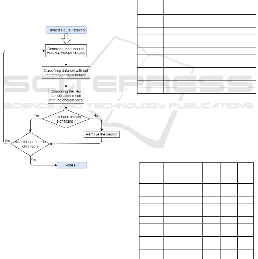
Figure 2 depicts a simple block scheme of the first
phase of the algorithm, which demonstrates the
removal of insignificant neurons for the purpose of
simplifying the result.
Figure 2: Pseudo scheme of the first phase of the algorithm.
5 GENERATION OF LENGTH
AND RANGE MATRICES
5.1 Data Length Matrices (DLMs)
As the network consist of important neurons only, it is
used for the generation of a matrix that contains
information on the number of examples classified in
different categories (Augasta, 2012). The rows within
the matrix correspond to different output categories of
the neural network. The number of columns is equal to
the number of input neurons. There are three versions
of this matrix. The first, shown in Table 1, contains
properly classified examples only. This is valuable for
the decision tree extraction. The main disadvantage of
this version, however, is not being able to provide the
necessary information on the most important input
neurons. As the significance of the neuron increases,
the number of correctly classified samples declines.
Therefore, the proper information from this neuron
decreases and can even descend to zero.
Table 1: DLM filled with properly classified samples.
Input 1 Input 2 Input 3 Input 4 Input 5
Class 1 1 1 0 4 1
Class 2 6 3 0 5 2
Class 3 8 8 0 4 1
Class 4 30 23 0 29 0
Class 5 91 98 0 94 0
Class 6 65 60 0 55 1
Class 7 77 96 0 59 1
Class 8 72 84 0 50 1
Class 9 28 44 3 21 1
Class10 5 6 0 5 0
Miss 438 398 818 495 813
Sum count 383 423 3 326 8
The second matrix type, shown in Table 2, is in
contrast to the first one, as it contains misclassified
samples only. It provides information on the most
significant neurons, but it is also used for the exclusion
of information that is regarded as incorrect. This matrix
type also grants a clear view of the most significant
inputs, as their absence generates a lot of mistakes.
Table 2: DLM with misclassified samples only.
Input 1 Input 2 Input 3 Input 4 Input 5
Class 1 0 1 0 0 0
Class 2 5 8 4 8 8
Class 3 16 6 4 16 13
Class 4 55 34 7 37 14
Class 5 101 86 19 98 59
Class 6 77 89 19 130 197
Class 7 98 89 122 122 157
Class 8 68 66 238 67 206
Class 9 17 19 278 17 127
Class10 1 0 126 0 32
Miss 383 423 4 326 8
Sum count 438 398 817 495 813
Decision Tree Extraction using Trained Neural Network
197
The third matrix type is shown in Table 3 and has
been used in this paper. It is comprised of properly
classified samples, together with those that are
misclassified. The samples are combined in order to
generate an overall view of the classification of the
data. In the last row one can observe an aggregated
value, i.e. the sum of elements from this column. This
sum is used for determining the significance of
information within the values.
Table 3: DLM filled with properly classified and
misclassified samples.
Input 1 Input 2 Input 3 Input 4 Input 5
Class 1 1 2 0 4 1
Class 2 11 11 4 13 10
Class 3 24 14 4 20 14
Class 4 85 57 7 66 14
Class 5 192 184 19 192 59
Class 6 142 149 19 185 198
Class 7 175 185 122 181 158
Class 8 140 150 238 117 207
Class 9 45 63 281 38 128
Class10 6 6 126 5 32
Miss 0 0 1 0 0
Sum count 821 821 820 821 821
After creating the matrix, values that do not
provide enough information are removed. Data that is
not sufficient for the tree extraction is truncated from
the matrix. A value is considered not informative if it
does not satisfy the following condition:
∗
(10)
where A is a threshold value within the range [0.05;
0.5]. It determines the minimum percentage of the
data needed for the corresponding range to remain in
the DRM. M
ij
is the elements in the row with index i
and the column with index j and Mc
j
is the sum of
elements in the column with index j. If M
ij
is lower
than the multiplication of the threshold value or lower
than the Mc
j
from this column, then the corresponding
range is no longer determinative. (Biswas, 2017)
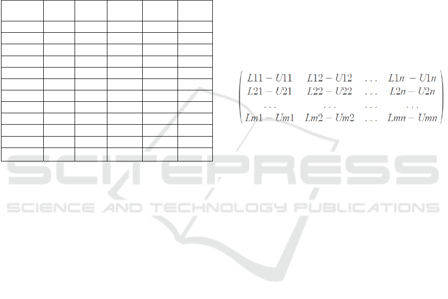
5.2 Data Range Matrices (DRMs)
After generating a data length matrix, the next step is
to construct a data range matrix (DRM), as shown in
Figure 3. The data range matrix is equal in size as the
data length matrix. However, its values represent
ranges that contain the minimum and maximum value
of each input neuron that has been classified into the
corresponding output category (Augasta, 2012).
Analogous to the DLM, the DRM can be divided into
three different types. The first includes ranges from
the correctly classified samples only. The second type
consists of ranges from misclassified samples only. It
is used to show what data should be excluded. The
third type contains ranges from both correctly and
incorrectly classified samples. Depending on the
approach used for the rule construction, different
matrices can be applied. There are two approaches
when it comes to rule construction – inclusion and
exclusion. The inclusion approach classifies data if
their properties lie within the values of the data range
matrix. Contrary to that, the exclusion approach
verifies whether the properties of the sample by
columns are excluded from the range. This study has
been observing the inclusion approach and has
therefore used the third data range matrix.
Figure 3: Abstract view of the Data Range Matrix.
where n in the number of input neurons and m is the
number of output categories.
The DRM matrix is used directly in the process of
extracting the rules for the decision tree. For this
purpose, all values that do not convey clear
information, as well as those that might blur the
results, are removed. For example, those values
where the distance between the upper and lower
limits
is close to the maximum possible distance to the
bottom limit. Such values cannot provide clear
information on the sample borders in this diapason.
For the purpose of generating a more refined tree,
values from the DRM that don’t have corresponding
counterparts in the DLM are also removed. The
reason for their removal lies in the fact that the sample
size, from which the ranges were provided, is not
sufficient enough.
6 CONSTRUCTION OF RULES
The tree is constructed from DRM ranges (Biswas,
2018) and uses easily obtained rules. Rules analyze
whether the input values lie within the corresponding
ranges. The following formulas give an abstract
representation of the extracted values, including
rules.
SMARTGREENS 2020 - 9th International Conference on Smart Cities and Green ICT Systems
198
if(L11 ≤ s1 ≤ U11 AND L12 ≤ s2 ≤ U12
AND...AND
L1n ≤ sn ≤ U1n)
then Class = 1
if(L21 ≤ s1 ≤ U21 AND L22 ≤ s2 ≤ U22
AND...AND
L2n ≤ sn ≤ U2n)
then Class = 2
... ... ...
if(Lm1 ≤ s1 ≤ Um1 AND Lm2 ≤ s2 ≤ Um2
AND...AND
Lmn ≤ sn ≤ Umn)
then Class = m
where L and U are lower and upper limits, N is the
number of input nodes and M the number of output
classes.
It is possible for the values of one sample to be
classified into several categories. This is corrected by
adding priorities to the output categories, which can
be achieved in two ways. The first is by prioritizing
categories according to the number of samples that
have been classified by the input network. The
second, more precise, approach is by prioritizing
categories according to the number of actual
informative ranges within the DRM. It can therefore
be stated that the most demanding category is the
first. If a particular sample conforms to the
conditions, no other processing will be required.
7 RULE UPDATE
Even though the extracted rules provide information
on the inner workings of the network, sometimes they
are not clear enough. The first step in improving an
extracted rule is by removing the redundant
verification. Rules can be improved by being
simplified and corrected. The simplification can be
compared to the network pruning, which is performed
at the beginning of the rule extraction. This is
achieved by classifying the sets with no verification
in the rule and by comparing the generated results
with the original ones. The absence of some
verification can improve the accuracy, since such
verifications would be considered redundant and are
therefore removed. Other verifications do not change
the accuracy of the rule but can be removed as well,
in order to create a simpler tree that is easier to
understand.
The second step regarding the improvement of
rules is redefining the upper and lower limits of
ranges. By shifting them, it is possible to generate
more accurate rules (Chakraborty, 2018). The
adjustment is performed busing a value that
represents the minimum difference between any two
possible values from the corresponding inputs. It is
possible to compare the original results with results
created by the adjusted rules to assess a negative
impact. In this way, both the adjustment is performed
and the accuracy increases.
8 RESULTS
Results can be presented in two different ways. The
first is as raw results of rules, which are short and
clear. The only drawback of rules is that they do not
provide visual representations. They do, however,
possess a form that is perfect for creating decision
trees and presenting them in a way that is easily
understandable. Rules are converted into a tree by
using the RBDT-1 method, known for making rule-
based decision trees (
Kalaiarasi, 2008). The RBDT-1
method is not the subject of this paper and is not
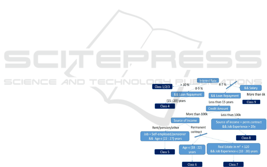
observed in detail. Figure 4 depicts a decision tree
generated from rules that have been extracted from a
neural network for the purpose of determining a credit
score. The tree is simplified for a better understanding
and a clearer view. The complexity of a tree grows as
the number of input neurons increases. The result is
highly dependable on the parameter used in formula
10. Extracted rules are cleaned with a coefficient of
0.2.
Figure 4: Rule-based decision tree.
The classification of the dataset that has been used
for the generation of the algorithm is based on
extracted rules. Several tests have been carried out
using different approaches of algorithms, including
various matrices and the including or excluding of
rules. Table 6 shows the different approaches and
their accuracy. Diff in % stands for the difference
between the original classification of the data set and
the classification after applying the rules.
Decision Tree Extraction using Trained Neural Network
199

Table 6: Results of the combination of different approaches.
DLM DRM RULE Diff in %
Right Right Include 16
Right Full Exclude 45
Full Right Include 16
Full Right Exclude 63
Full Full Include 27
Wrong Full Include 19
9 CONCLUSIONS
One of the main disadvantages of neural networks is
people’s inability to fully comprehend their workings.
Their black box nature makes them useless in cases
where the process of classification is important and
must be presented in an observable and understandable
way. The algorithm described in this paper extracts
rules from a trained neural network and presents them
in the form of a decision tree. In general, decision trees
are easy to understand and memorize.
ACKNOWLEDGEMENTS
This work is supported by Eurorisk Systems Ltd.
REFERENCES
Antonov, A., Nikolov, V., 2018. Analysis of Scoring and
Rating Models using Neural Networks. Journal of
International Scientific Publications, Economy &
Business, Vol. 12/2018, ISSN 1314-7242, pp. 105-118.
Jivani, K., Ambasana, J., Kanani, S., 2014. A survey on rule
extraction approaches-based techniques for data
classification using NN. Int. J. Futuristic Trends Eng.
Technol. 1(1), 4–7.
Craven, M, Shavlik, J., 1999. Extracting Tree-Structured
Representations of Trained Networks. Adv Neural
Inform Process Syst. 8.
Biswas, S., Chakraborty, M., Purkayastha, B., 2018. A rule
generation algorithm from neural network using
classified and misclassified data. International Journal
of Bio-Inspired Computation. 11.60.10.1504/IJBIC.
2018.090070.
Augasta, M., Kathirvalavakumar, G., 2012. Reverse
Engineering the Neural Networks for Rule Extraction
in Classification Problems. Neural Processing Letters,
35(2), pp. 131–150.
Biswas, S. et al., 2017. Rule Extraction from Training Data
Using Neural Network. International Journal of
Artificial Intelligence Tools, World Scientific.
26.10.1142/S0218213017500063.
Chakraborty, M., Biswas, S., Purkayastha, B., 2018. Rule
Extraction from Neural Network Using Input Data
Ranges Recursively. New Generation Computing.
10.1007/s00354-018-0048-0.
Kalaiarasi, S., Sainarayanan, G., Chekima, A., Teo, J.,
2008. Investigation of Data Mining Using Pruned
Artificial Neural Network Tree. Journal of Engineering
Science and Technology. 3.
Setiono, R., Baesens., B., Mues, C., 2008. Recursive Neural
Network Rule Extraction for Data with Mixed
Attributes. IEEE Transactions on Neural Networks,
19(2), pp. 299–307.
Quinlan, J. R., 1993. Programs for Machine Learning.
Morgan Kaufman, San Mateo.
Chakraborty, M., Biswas, S., Purkayastha, B., 2018.
Recursive rule extraction from NN using reverse
engineering technique. New. Gener. Comput. 36, 119.
https://doi.org/10.1007/s00354-018-0031-9.
Filer R, Sethi, I., Austin, J., 1997. A comparison between
two rule extraction methods for continuous input data.
In: Proceedings of neural information processing
systems, rule extraction from trained artificial neural
networks workshop, pp 38–45.
SMARTGREENS 2020 - 9th International Conference on Smart Cities and Green ICT Systems
200
