Prediction of Spatiotemporal Distributions of Transient Urban

Populations with Statistics Gathered by Cell Phones

Toshihiro Osaragi

a

and Ryo Hayasaka

School of Environment and Society, Tokyo Institute of Technology, 2-12-1 Ookayama, Meguro, Tokyo, Japan

Keywords: Moving People, Spatiotemporal Distribution, Mobile Spatial Statistics, Konzatsu-tokei

®

, Person Trip Survey,

Maximum Likelihood Method.

Abstract: There is a growing demand for data that facilitate highly accurate understanding of the spatiotemporal

distribution of both moving and static occupants in urban areas. Currently, a large amount of population data

are available, however none of the data provide an accurate understanding of the numbers and

departure/arrival locations of moving people using detailed units of space and time. In this paper, after

evaluating the advantages and disadvantages of existing population statistics, including Mobile Spatial

Statistics, Konzatsu-tokei®, and Person Trip survey data, we propose a method based on maximum likelihood

method is investigated for using their strengths to best advantage and compensating for weaknesses. The

proposed method is then validated by comparing with another flow data, which featured spatiotemporal data

including departure/arrival locations, and demonstrate that the present procedure provides accurate estimates

for population flows. This study makes it possible to analyse urban regions from new and never-before

employed points of view by identifying the number of transient occupants and their travel directions at any

time on high level of detail.

1 INTRODUCTION

1.1 Research Background

There has recently been growing interest in the

observation and analysis of people’s movements on a

large map scale, with the goals of mitigating

crowding and avoiding risks at large-scale public

events, identifying appropriate initial responses, and

guiding evacuation during the aftermath of major

earthquakes, and for area marketing in the

commercial and travel industries. Since distribution

of population in the largest conurbations fluctuates

rapidly with the advance of public transportation

systems, the conventionally used “static” data such as

previously gathered population statistics are of only

limited value in analyses. This has resulted in a need

for a technological method to map dynamic

population distributions on a large map scale at any

desired time. Namely, we need a method which

enables us to identify the number of transient

occupants and their travel directions at any time, on

large map scales for the analyses on human activities

a

https://orcid.org/0000-0002-6327-3976

in urban areas from new and never-before employed

points of view.

1.2 Existing Research and Population

Statistics

A variety of statistical analyses of population have

been created and are available for use by parties

observing the behavior of static and transient

populations in urban areas. Table 1 shows examples

of data that have been useful for wide areas.

The first of these is the set of regional grid-cell

statistics based on the long-established national

census of Japan. It includes the population, number of

households, levels of schooling, and much other

information. Only a few national censuses around the

world offer such a rich store of demographic

information. However, it is conducted at 5-year

intervals and based on residential location, so it is a

static population distribution.

Person Trip survey data (PT data) focus on

people’s spatial motions. PT data are based on

responses to questionnaire surveys and provide much

Osaragi, T. and Hayasaka, R.

Prediction of Spatiotemporal Distributions of Transient Urban Populations with Statistics Gathered by Cell Phones.

DOI: 10.5220/0009325700330044

In Proceedings of the 6th International Conference on Geographical Information Systems Theory, Applications and Management (GISTAM 2020), pages 33-44

ISBN: 978-989-758-425-1

Copyright

c

33

Table 1: Characteristics of population statistics.

information, including the sex, age classification,

purpose of movement/stay, means of transportation,

departure/arrival locations and times, etc. Osaragi et

al. (2009, 2012, 2015) has used the PT data and

building geographic information system (GIS) data to

construct a model for estimating how many people

are statically occupying a given spatial unit of a city

at any given time, and in models for estimating the

spatiotemporal distribution of transient city

occupants (railroad and automobile users).

Another proposed approach is to estimate PT data

for weekends and holidays by using a time use survey

(Osaragi, 2016). Numerous studies exploiting PT data

have been published in the civil and transportation

planning fields. For example, researchers have used

spatiotemporal interpolation to examine problems in

spatial units (Sekimoto et al., 2011) and have

combined observed data of differing types to

reevaluate trips as an approach to the problem of low

sampling fraction (Nakamura et al., 2013). Another

study combined the national census with time use

surveys to construct daily mobility and activity data

(Hidaka et al., 2016). These studies were all attempts

to compensate for the shortcomings of PT data and

provide useful background for this study, which has

the same theme. However, the PT data were taken at

10-year intervals, so they do not help in overcoming

the lack of fresh data.

In counterpoint to the above methods, recent

studies have employed location data from cell phone

records to create and provide spatiotemporal data for

people’s locations. For example, Mobile Spatial

Statistics (MSS) from mobile phones provide

regional populations in grid-cell units at any desired

time, which are provided by NTT DoCoMo Inc.

Mobile terminals connect to the base stations in a

certain time interval in order to maintain the

mechanism that allows mobile terminals to be paged

at any time and any place. Location data is estimated

using the locations of coverage area of base stations

(the grid-cell) (Okajia et al., 2013). These are

population statistical data, the number of cell phones

using the cellular network, and incorporate the

penetration ratio among cell phones operated by

DoCoMo (rate of DoCoMo users to the total number

of mobile phone users). The spatial information (each

user’s location) is presented as the grid-cell, which is

generally about 500 m by 500 m grid. MSS is a

registered trademark by NTT DoCoMo. Seike et al.

(2011) validated the reliability of MSS (distribution)

and showed that it is also possible to use these

statistics for transportation and urban planning.

Osaragi and Kudo (2019) proposed a method for

estimating the purpose of the buildings people

stopped in and their reasons for staying there by

combining MSS (distribution) with PT data. The

same studies have also been carried out in foreign

countries (Deville et al., 2014; Ratti et al., 2006).

However, MSS (distribution) do not make it possible

to distinguish between persons who are moving and

those who are static. Arimura et al. (2016) have

published an extremely interesting estimate of the

population inflows into buildings, but were not able

to identify their movement directions.

New data regarding the numbers of transient city

occupants and their trajectories have been compiled

and offered in response to the increasing need for

these data. Konzatsu-tokei

®

(KT) are the locations of

GISTAM 2020 - 6th International Conference on Geographical Information Systems Theory, Applications and Management

34

the cell phones, provided under the consent of the

user by an application provided by NTT DoCoMo.

These are provided as overall data, with statistical

information added. The location data are transmitted

every 5 minutes along with Global Positioning

System (GPS) data (latitude and longitude), and any

information that would identify the user is excluded.

This application is a part of the DoCoMo map and

navigation service (map application and current

location guide). Since those data were taken from an

application loaded just by certain users, however, the

sampling fraction was low, and the accuracy is

unstable in regions with low population densities

(Kamada, 2017). Additionally, MSS (flow) data are

based on the departure/arrival location information

obtained from cell phones, just as MSS (distribution)

data are. MSS (flow) are provided by NTT DoCoMo

Inc. These are population statistical data, the number

of cell phones using the cellular network, and

incorporate the penetration ratio among cell phones

by DoCoMo. These data are the total numbers of

travelers who departed from one location and moved

to another. Phone users who have not moved (that is,

static occupants) are not included in these data. These

provide a greater sampling fraction and higher

accuracy than KT, but since they are taken at 60-

minute intervals, it is difficult to construct trajectories

for people who move quickly. These data are also

obscured by the process of anonymization (Ishii et al.,

2017).

Agoop data (point-type floating population data)

are location information from users whose cell

phones are equipped with a special application. These

data are provided without reference to the user’s cell

phone carrier, but again, the sampling fraction is low

(Matsubara, 2017). Turning overseas, however,

Calabrese et al. (2011) has proposed a method for

tabulating departure/arrival location data which can

accommodate daily and seasonal fluctuations, while

Iqbal et al. (2014) has proposed a method for creating

departure/arrival location data by combining the

transmission histories of cell phones with actual data

from sampling surveys. Nevertheless, these

approaches do not generate data on a large map scale,

and it would be impractical to use them when carrying

out actual surveys in a large city due to the cost

involved.

Thus, each of the existing datasets for transient

and static individuals has its own advantages and

disadvantages from the viewpoints of time units,

spatial units, sampling fraction, etc., and each

imposes a variety of limitations on research objects

and methods. This study investigates a method for

creating a spatiotemporal data structure of transient

city occupants by providing their numbers and their

directions of travel. The data were integrated while

employing the useful aspects of each of the

population statistics types such as arbitrary time units,

large-map-scale units, and high sampling fraction,

and compensating for their defects.

2 DATA INTEGRATION

METHOD

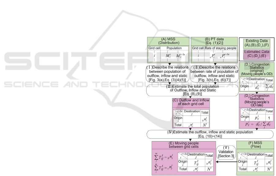
2.1 Overview of Integration Method

The integration process is summarized in Fig. 1. The

main variants are shown below:

a

n

i

t

,

a

P

i

t

: Number of people and population fraction

occupying grid-cell i

b

n

i

t

,

b

P

i

t

: Number of people and population fraction

exiting grid-cell i

c

n

i

t

,

c

P

i

t

: Number of people and population fraction

entering grid-cell i

Figure 1: Integration of multiple demographic datasets.

This report employs MSS (distribution) data,

which consists of detailed records featuring high

sampling fractions and precise temporal and spatial

units, as the basic information expressing the

spatiotemporal population distribution. However,

population M

i

t

(Fig. 1(A)) occupying cell i at time t,

which is obtained from the MSS (distribution), fails

to distinguish between transient and static occupants.

Prediction of Spatiotemporal Distributions of Transient Urban Populations with Statistics Gathered by Cell Phones

35

Therefore, we attempted to make this distinction by

defining the fraction of static occupants (static

occupant fraction

a

P

i

t

, Fig. 1(B)) obtained from the

PT data using the following method. M

i

t

, obtained

from the MSS (distribution), was imposed as a

constrain and a maximum likelihood algorithm was

written to hold the sum of the number of static,

entering, and exiting occupants to M

i

t

. This provided

estimates for

a

n

i

t

, the number of static occupants,

b

n

i

t

,

the number of exiting occupants, and

c

n

i

t

, the number

of entering occupants (Fig. 1(C)).

Next, data for spatial motions were compiled from

KT, which contains detailed spatiotemporal

information about departure/arrival locations and

times. The fraction of population motions between

cells i and j during time span t to t+

Δ

t is denoted p

ij

t

(Fig. 1(D)).

Last, the maximum likelihood estimator T

ij

t

for the

number of individuals moving between grid-cells i

and j is found via the inter-grid-cell motion fraction

p

ij

t

, using the number of individuals leaving grid-cell

i,

b

n

i

t

, and the number of individuals entering grid-cell

i,

c

n

i

t

, in the criterion (Fig. 1(E)).

2.2 Method for Estimating Fractions of

Static and Transient Occupants

It is quite common for the population (static and

transient numbers) of any given region to fluctuate

widely from year to year, due to redevelopment and

other factors. In contrast, individual movement

patterns, whether these people are static or transient,

vary most dramatically with clock time and day of the

week (Osaragi, 2012). For this reason, one would

expect the fractions represented by static and transient

occupants to be relatively stable from year to year.

Therefore, in this study, PT data was used to estimate

these fractions, as it is the only dataset that allows

distinguishing between static and transient occupants.

First, based on the consideration that the numbers

of static and transient occupants could be proportional

to the floor area of a building, depending on the

building’s use classification (Osaragi, 2012), the

static and transient occupants indicated by the PT data

were distributed proportionately among all of the

buildings. In other words, the information about

spatial motion incorporated in the PT data was used

to identify

uv

S

kl

t

, the number of people passing

between buildings of use classifications u and v,

located in small zones k and l, during time span t to

t+Δt. It was assumed that the transient occupants

moved at a constant speed over the shortest route on

a transient irregular network (TIN) between the

centers of gravity of their starting and destination

zones; the times t and t+Δt in the occupied small

zones k and l were identified (Fig. 2). The proportions

of floor areas of the buildings in grid-cells i and j in

zones k and l,

u

A

i

/

u

A

k

and

v

A

j

/

v

A

l

, were found using the

GIS data for the buildings, and the number of

transient individuals between grid-cells i and j during

time span t to t+Δt, s

ij

t

, was calculated using the

equation below. The reader’s attention is directed to

s

ii

t

, which designates individuals moving within grid-

cell i:

uv

vj

tt

ui

ij

kl

uvkl

uv

kl

R

sS

RR



=××







(1)

Last, the number of transient occupants s

ij

t

and the

number of static occupants s

i

t

in grid-cell i (who did

not move at all) were used to find the static occupant

fraction

a

P

i

t

in grid-cell i during time span t to t+Δt.

(2)

Figure 2: Estimation of traveling route between OD zones.

2.3 Method for Estimating Grid-cell

Inflows and Outflows

For the populations M

i

t

and M

i

t+Δt

in grid-cell i

obtained from the MSS (distribution), relational

expressions Eqs. (3)-(5) below provide estimates of

the number of people not moving within grid-cell i

(number of static occupants)

a

n

i

t

, the number of

people leaving the zone

b

n

i

t

, and the number of people

entering the zone

c

n

i

t

during time span t to t+Δt (Fig.

1(I), Fig. 3(a)).

(3)

(4)

(5)

Suppose motions in grid-cell i during time span t to

t+Δt are summarized as the following four cases (Fig.

3(b)).

(i) The individual remains in grid-cell i during time

span t to t+Δt.

a

j

t

i

tt

iij

s

P

s

=

+



bc

tt t

ii

tt

ii

M

Mnn

+Δ

=−+

ab

tt t

iii

nnM+=

ac

tt tt

ii i

nnM

+Δ

+=

GISTAM 2020 - 6th International Conference on Geographical Information Systems Theory, Applications and Management

36

Figure 3: Relationships between moving people and static

people.

(ii) The individual moves out of grid-cell i to another

grid-cell.

(iii) The individual moves from another grid-cell into

grid-cell i.

(iv) The individual passes through (into and out of)

grid-cell i during time span t to t+Δt.

Then static occupants correspond to (i), exiting

occupants can be (ii) or (iv), and entering occupants

can be (iii) or (iv). The following expression

describes the relationships between the static

occupant fraction

a

P

i

t

and the population fraction

exiting grid-cell i

b

P

i

t

, and between the static occupant

fraction

a

P

i

t+Δt

and the population fraction entering

grid-cell i

c

P

i

t

(Fig. 1(II)): The details are described in

Appendix (A).

(6)

(7)

When the populations M

i

t

and M

i

t+Δt

and the static

occupant fractions

a

P

i

t

and

a

P

i

t+Δt

are known, the

following equations for the maximum likelihood

estimator for the number of static occupants

satisfying the criteria (Eqs. (3)-(5), Eqs. (6) and (7))

can be derived:

(8)

(9)

Once the number of static occupants

a

n

i

t

in grid-cell i

during time span t to t+Δt has been found, the number

of people exiting grid-cell i

b

n

i

t

and the number of

people entering grid-cell i

c

n

i

t

can be calculated (Fig.

1(III)).

2.4 Method for Calculating Number of

Transient Occupants

The numbers of people leaving (

b

n

i

t

) and entering

(

c

n

i

t

) are used in criteria for the hourly calculations of

population distribution. Additionally, the inter-grid-

cell motion fractions p

ij

t

between grid-cells i and j

during time span t to t+Δt can be calculated from KT.

These are used to calculate the maximum likelihood

estimator for individuals moving between grid-cells i

and j during time span t to t+Δt.

Between the numbers of people leaving and

entering and the number of individuals moving

between grid-cells T

ij

t

, we establish Eqs. (10) and (11)

(Fig. 1(E)). (Note that m denotes the number of grid-

cells.)

(10)

(11)

The number of individuals moving between grid-

cells T

ij

t

is calculated as follows, employing the inter-

grid-cell motion fractions p

ij

t

obtained from the KT

under the above the maximum likelihood estimators

providing the highest values for the occurrence

probabilities. The details are described in Appendix

(B).

(12)

(13)

(14)

Variables A

i

t

and B

j

t

are mutually dependent, but

arbitrary starting values are chosen for a converging

calculation, and this will provide the unique value for

the number of individuals moving between grid-cells

T

ij

t

.

1

ab

tt

ii

PP+=

1

ac

tt t

ii

PP

+Δ

+=

()()

2

4

2

a

t

i

ttt ttt ttt

ii ii ii

MM MM PMM

n

P

+Δ +Δ +Δ

−−

=

++

1

aa

ttt

ii

ttt

ii

PP

P

PP

+Δ

+−

=

m

b

j

t

ij

t

i

nT=



m

c

i

t

ij

t

j

nT=



t

ij

ttt

ij i j

TpAB=××

b

m

t

ij

j

t

i

t

j

t

i

n

A

pB

=



c

m

t

ij

i

t

j

t

i

t

j

n

B

pA

=



Prediction of Spatiotemporal Distributions of Transient Urban Populations with Statistics Gathered by Cell Phones

37

3 CALCULATION AND

VALIDATION OF NUMBER OF

TRANSIENT CITY

OCCUPANTS EMPLOYING

ACTUAL DATA

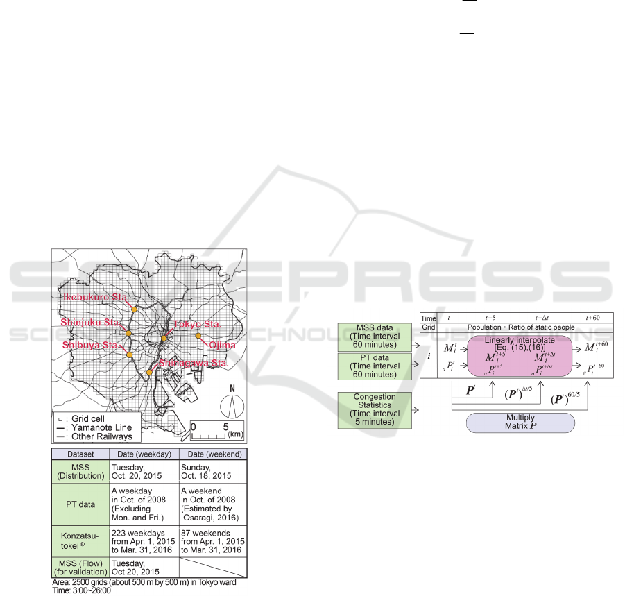
3.1 Study Region and Data

The region used for analysis was the Tokyo 23-ward

area (Fig. 4), divided into a grid-cell of spatial units

500 m by 500 m grid. Data from MSS (distribution)

on a weekday and a weekend day in October were

used. The location of each individual was estimated

from the PT data at 60-minute intervals, and the PT

data from the weekend day was assessed using time

use survey results (Osaragi, 2016). Since the

sampling rates for KT are low, datasets from multiple

days were combined. Days when anomalies occurred

due to natural causes and when there were large

public events were excluded, leaving approximately

half a year, and data from this set were extracted to

create one day’s worth each of weekday and weekend

data.

Figure 4: Study area and data used in this paper.

3.2 Pre-processing of Data for

Integration of Time Intervals

Data were generally extracted from MSS

(distribution) at 60-minute intervals, but from KT,

they were extracted at 5-minute intervals. The

following process was performed in order to integrate

those intervals.

First, the grid-cell i population M

i

t+Δt

and static

occupant fraction

a

P

i

t+Δt

at time t+Δt (Δt=1, 2, …, 60)

were estimated by linear interpolation using the

following equations (t+60 means 60 minutes after

time t):

(15)

(16)

The numbers of people moving between grid-cells

i and j at 5-minute intervals in KT, d

ij

t

, were obtained

by calculations with the data taken at 60-minute

intervals. The 5-minute means were evaluated using

the inter-grid-cell motion fraction p

ij

t

(Δt=5 minutes)

in the following equation:

(17)

If it is assumed that the inter-grid-cell motion

fraction during any arbitrary time span

Δ

t is the

simple Markov type, then the motion fraction matrix

P

t

, whose elements are the inter-grid-cell motion

fraction p

ij

t

, can be obtained by multiplying the

motion fraction matrix by Δt/5 (Fig. 5).

Figure 5: Unifying time interval of datasets.

3.3 Validation of Accuracy of

Estimates

No data exist that clearly show the numbers of

transient city occupants in fine temporal or spatial

units, but comparing results with the MSS (flow),

which actually do offer rather fine detail, allows the

accuracy of the proposed procedure to be validated.

First, since trips in the MSS (flow) are anonymized

when there are few travelers, it is inappropriate to

compare the numbers of people per se. Instead, the

ratios between the numbers of people exiting

b

n

i

t

and

entering

c

n

i

t

(Δt=60 minutes) are compared. Here, the

spatial grid-cell unit was widened to 1 km in order to

minimize the influence of anonymization.

()

60

tt t t t

ii ii

t

M

MMM

+Δ +

Δ

=+ −

()

60

aa aa

tt t t t

ii ii

t

P

PPP

+Δ +

Δ

=+ −

/

tt t

ij ij ij

j

pd d=



GISTAM 2020 - 6th International Conference on Geographical Information Systems Theory, Applications and Management

38

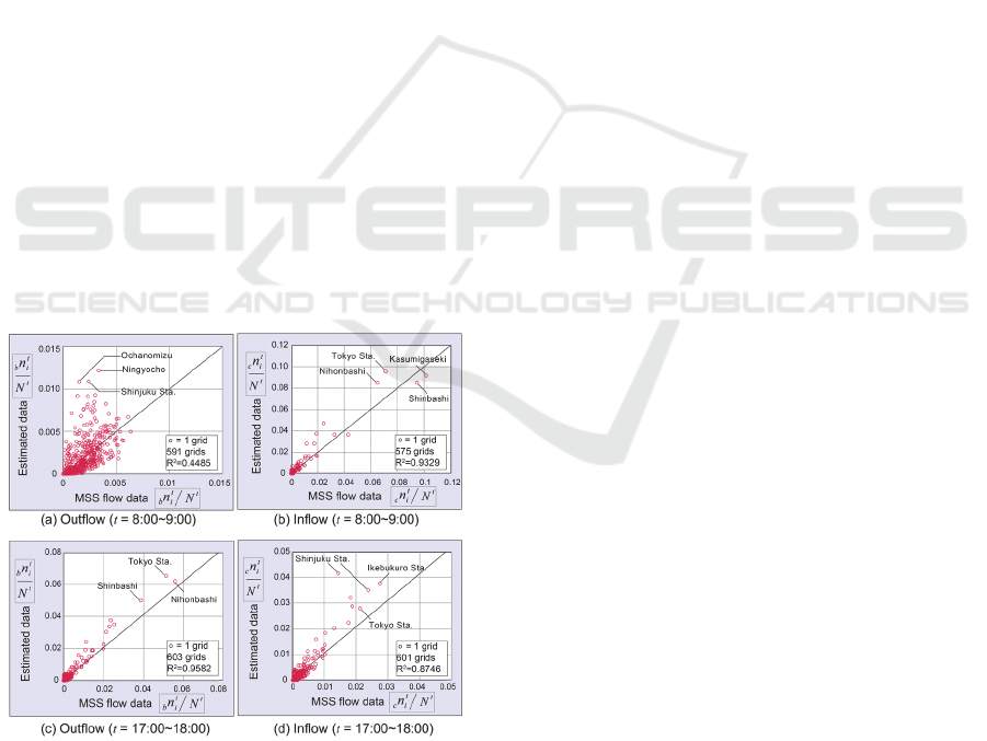
During the 08:00-09:00 hour, when numerous

people are commuting to work or school (Fig. 6(a)),

the outflows are people leaving residential areas in all

possible directions, so the above ratios are not high.

In general, since the proportion of numerical errors

are relatively large for small values, the result shows

low correlation. On the other hand, examining the

people who are entering grid-cells (Fig. 6(b)), the

reader can see that this approach provided particularly

accurate predictions of the tendencies for high

numbers of commuter inflow at grid-cells in the

vicinity of large train stations. Turning to the 17:00-

18:00 hour, when many are returning home (Fig. 6(c),

(d)), both inflows and outflows are seen to be

accurately predicted.

However, a close examination of Fig. 6 also

reveals some overestimates in all estimates for

outflow/inflow in the morning/evening. One of the

reasons for this was the data based on

departure/arrival locations in the MSS (flow)

information. This is because the numbers of

individuals were counted only at the departure and the

arrival locations. In other words, since the people

passing through a grid-cell during a 5-minute period

were not counted in MSS (flow), the actual

population was undercounted by that amount. In this

procedure, in contrast, the much more accurate MSS

(distributions) were employed in criteria for

calculating the number of people passing through a

grid-cell. This highlights the potential of this

procedure to provide highly accurate calculations.

Figure 6: Validation by using MSS flow data.

4 ANALYSIS OF SPATIAL

MOTION DISTANCES

TRAVELLED BY TRANSIENT

CITY OCCUPANTS

4.1 Spatial Distributions of

Inter-grid-Cell Crossing Numbers

per Unit Time

This procedure enables prediction of static, transient,

and incoming populations at any desired time interval

(Fig. 7(c)), parameters which are not available from

the existing data from MSS (distributions) (Fig. 7(a)).

For example, there is little difference in the spatial

distributions of static, transient, or incoming

populations during the 5 minutes from 08:00 to 08:05,

and we can see high concentrations near the large

train stations. Over the 60 minutes between 08:00 and

09:00, however, the static populations become quite

widely distributed. The reader can see that exiting

populations show high numbers near Shinjuku

Station, which is a commonly used stop for transfers

between lines, while there are large inflows around

the main stations of lines connecting to the Yamanote

Line. Thus, this procedure allows close examination

not only of the total population but also separate

examinations of the differences between the static,

outflowing, and inflowing populations, and these

examinations can take place over any desired time

units.

Now,

let us turn to some observations about the

distributions of inflows and outflows on a special

grid-cell in order to clarify some characteristics of the

Tokyo population. Focusing first on the grid-cell

surrounding Shinagawa Station, the average numbers

of people exiting and entering the station at 5-minute

intervals between 08:00 and 09:00 obtained from KT

are shown in Fig. 7(b). Many of the exiting people

leave in the direction of Tokyo Station, and many of

the incoming people are from Kanagawa Prefecture.

This combination can easily be read as early-morning

commuting to work. Since the sampling fraction in

KT is low, however, it is difficult to make an accurate

estimate of the number of people. Additionally,

estimates can only be made about locations with large

transient populations.

Examining the predictions of the proposed

procedure for outflow from and inflow to Shinagawa

Station (Fig. 7(d)), we found they were similar to the

results from KT during the 5 minutes of 08:00-08:05

(Fig. 7(d)(1),(2)), but the reader can see that during

the 60 minutes of 08:00-09:00, inflow originated

from a wide region and was not limited to that from

Prediction of Spatiotemporal Distributions of Transient Urban Populations with Statistics Gathered by Cell Phones

39

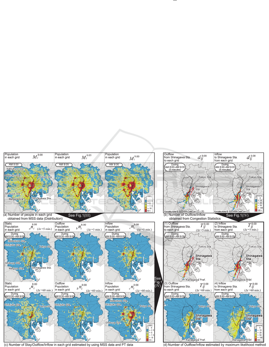
Kanagawa Prefecture (Fig. 7(d)(3),(4)). As this

example demonstrates, this procedure is capable of

indicating the numbers of exiting and incoming

people and their trajectory directions over a variety of

time spans. Therefore, it can be used for a variety of

analyses that require data about static and transient

people in the city.

4.2 Analysis of Region based on

Temporal Fluctuations of Inflow

and Outflow

Next, we attempted to identify the characteristics of a

region by the variation with time of exiting and

incoming individuals. Figure 8 shows how the

numbers of people exiting

b

n

i

t

and entering

c

n

i

t

6

regions (grid-cells) varied with time (Δt=60 minutes).

Here, the location on the graph found from the

outflow

b

n

i

t

and the inflow

c

n

i

t

was graphed and is here

called the “pole”; the surface area D

i

of the closed

region generated by observing the translation of the

pole as the clock time was calculated as follows:

(18)

The value of D

i

in this calculation was positive

when the pole shifted in the clockwise direction and

negative when it shifted counterclockwise.

D

i

took a positive value in the densely built

commercial and office areas around Tokyo Station,

Shinagawa Station, and others, as the rotation of the

pole was generally clockwise. Many people

commuted to these areas in the morning, while there

was little outflow or inflow during the day. They

resembled each other in that greater numbers of

people began to leave for home in the late afternoon

(Fig. 8(a),(b)), but the reader can see that Tokyo

Station saw greater numbers of people from 09:00 to

18:00. Shinjuku Station (a commercial and office

district, as well as a station hosting many transfers

between lines) showed the same tendencies in the

morning, but saw greater numbers of people exiting

and entering during the day and in the late afternoon;

due to this, the closed district had a larger area (Fig.

8(c)).

Figure 7: Spatial distribution of Static/Outflow/Inflow population grasped by using MSS data, Konzatsu-tokei

®

(KT) and

estimated results.

()()

1

2

ibbcc

t

tttttt

iiii

Dnnnn

+Δ +Δ

=−+



GISTAM 2020 - 6th International Conference on Geographical Information Systems Theory, Applications and Management

40

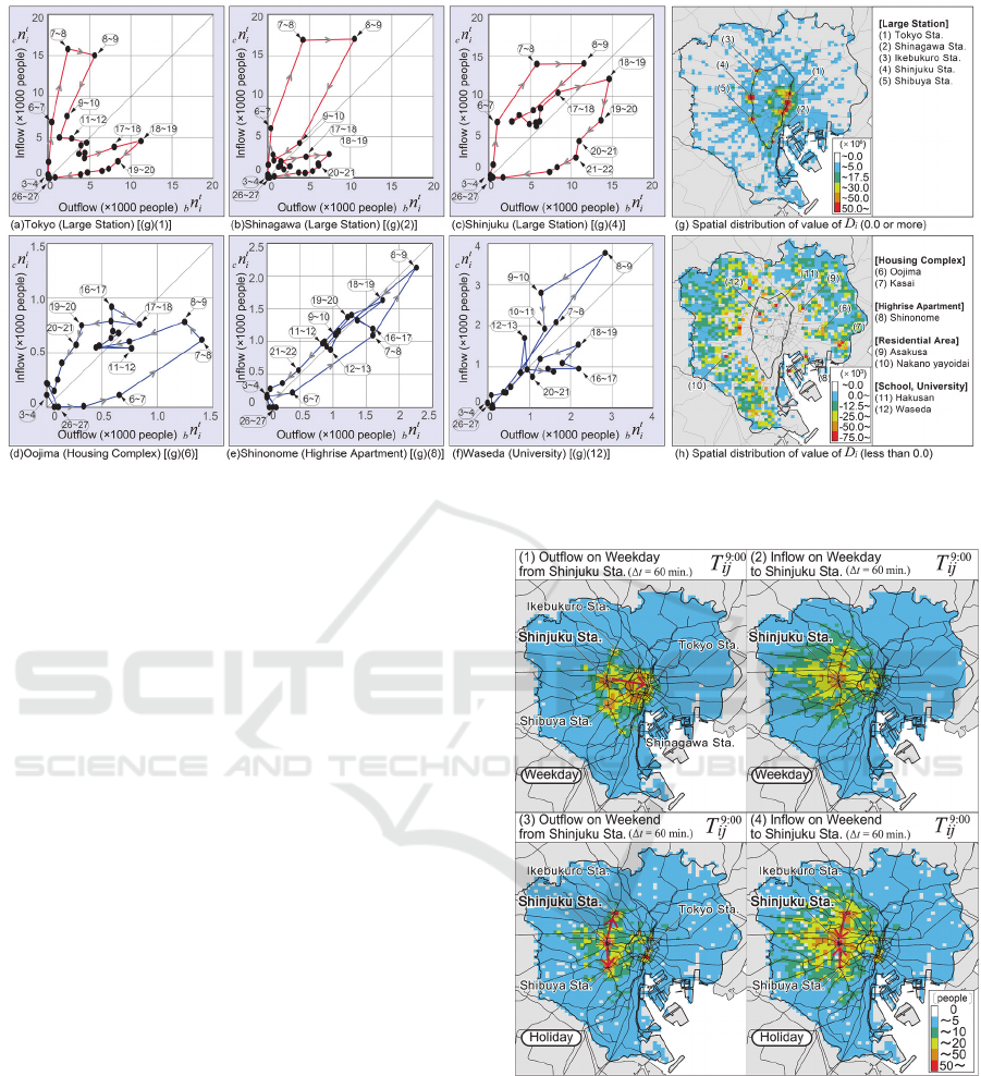
Figure 8: Temporal change in the relation between outflow population and inflow population and Spatial distribution of value

of Di.

In Oojima (an area with large-scale housing),

however, exiting people were in the overwhelming

majority in the morning and inflow increased from

the late afternoon on, resulting in a D

i

with a large

negative value (Fig. 8(d)). The same pattern was

found in Shinonome (an area with high-rise

condominiums), but because the numbers of people

exiting and entering the region changed similarly, the

closed region was longer but thinner than in Oojima

(Fig. 8(e)). Thus, the poles in such regions with large

residential areas tend to rotate in a counterclockwise

direction, resulting in negative D

i

.

Figures 8(g) and (h) show the spatial distributions

and the areas D

i

of the closed regions when the same

calculations were performed at other locations (grid-

cells). Grid-cells with positive values crowd the areas

adjacent to the rail routes. This was particularly true

along routes connecting to the main stations of the

Yamanote Line, where the positive values were high.

On the other hand, grid-cells with strongly negative

values had many groups of high-rise condominiums,

large-scale residential neighborhoods, universities,

and the like. These areas saw gradually increasing

inflows of population from the morning into the

daytime (Fig. 8(f)).

4.3 Directions of Travel on Weekdays

and on Weekends

Next, we make some observations about the

directions of travel of the users of Shinjuku Station

between

09:00

and

10:00

on

weekday

and

weekend

Figure 9: Spatial distribution of the estimated moving

population from/to Shinjuku Sta. between 9:00 and 10:00

on weekday and weekend.

exiting the grid-cell on weekday mornings indicate

that many proceed in the direction of Tokyo Station

(Fig. 9(1)). On weekend mornings, in contrast, most

outflows are in the directions of other stations

including Shibuya and Ikebukuro, which are densely

built commercial areas (Fig. 9(3)). Thus, we see that

weekend mornings showed a higher diversity of

Prediction of Spatiotemporal Distributions of Transient Urban Populations with Statistics Gathered by Cell Phones

41

directions of travel than weekday mornings. Further

examination of the spatial distributions of inflow to

Shinjuku Station revealed that the same grid-cells

furnished most of the inflows on both weekdays and

weekends, but there were higher inflows from

Shibuya Station and Ikebukuro Station on weekends

(Fig. 9(4)).

5 SUMMARY AND

CONCLUSIONS

This study has proposed a method for estimating the

spatiotemporal distribution of static and transient

populations of urban areas by using population

statistics created from the location information for

users of cell phones. The advantages and

disadvantages of the various population statistics

available were evaluated and methods were

investigated for integrating the data while using their

strengths to best advantage and compensating for

weaknesses. MSS (distribution), with its high

numbers of samples and high accuracy, was

employed in a criterion for population distribution

data consisting of summed numbers of transient and

static individuals.

Additionally, KT, with their low sampling rate but

detailed information about individuals’ motions, were

used for generating the inter-grid-cell motion fraction

data. These were applied to a method constructed to

evaluate the maximum likelihood estimator for

calculating the numbers of people exiting or entering

a given grid-cell. These were then compared with the

MSS (flow), which featured spatiotemporal data

including departure/arrival locations to verify that the

present procedure provides accurate estimates for

these population flows.

Next, we attempted analysis of regions by

calculating the numbers of transient occupants and

their directions of motion, per unit of time, in several

regions. This was found to provide a quantitative

grasp of the characteristics of transient urban

occupants, which had been difficult to identify

previously. For example, differences between

weekdays and weekends in the characteristics of

motion were noted, and large differences between

otherwise similar areas with commercial and office

concentrations in occupants’ travel directions were

identified.

The procedure proposed in this study makes it

possible to identify the number of transient occupants

and their travel directions at any time, on large map

scales, by using the constructed spatiotemporal data

for both static and transient urban occupants, and to

obtain and use these basic data to analyze urban

regions from new and never-before employed points

of view.

In further research, we would like to undertake a

comparison of our proposed approach with relevant

studies conducted in other countries addressing the

same topic of people’s movements. Also, using our

proposed method, we would like to construct a model

to evaluate the influence of large-scale public events

or natural disaster on people’s movements, which

assists mitigating crowding and avoiding risks,

identifying appropriate initial responses, and guiding

evacuation.

ACKNOWLEDGEMENTS

This paper is part of the research outcomes funded by

KAKENHI (Grant Number 17H00843). A portion of

this paper was published in Osaragi and Hayasaka

(2019). The authors wish to express their sincere

thanks for valuable comments and suggestions from

anonymous reviewers of GISTAM 2020.

REFERENCES

Osaragi, T. (2009). Estimating Spatio-Temporal

Distribution of Railroad Users and Its Application to

Disaster Prevention Planning, 12th AGILE Conference

on Geographic In-formation Science, Lecture Notes in

Geoinformation and Cartography, Advances in

GIScience, Springer, 233-250.

Osaragi, T., Hoshino, T. (2012). Predicting Spatiotemporal

Distribution of Transient Occupants in Urban Areas,

15th AGILE Conference on Geographic Information

Science, Lecture Notes in Geoinformation and

Cartography, Bridging the Geographic Information

Sciences, Springer, 307-325.

Osaragi, T. (2015). Spatiotemporal Distribution of

Automobile Users: Estimation Method and

Applications to Disaster Mitigation Planning, 12th

International Conference on In-formation Systems for

Crisis Response and Management (ISCRAM 2015),

Proceedings of the ISCRAM 2015 Conference,

ISCRAM 2015 Organization, May. 2015.

Osaragi, T. (2016). Estimation of Transient Occupants on

Weekdays and Weekends for Risk Exposure Analysis,

13th International Conference on Information Systems

for Cri-sis Response and Management (ISCRAM 2016),

Proceedings of the ISCRAM 2016 Conference,

ISCRAM 2016 Organization, May. 2016.

Sekimoto, Y., Shibasaki, R., Kanasugi, H., Usui, T. and

Shimazaki, Y. (2011). PFlow: Reconstructing People

GISTAM 2020 - 6th International Conference on Geographical Information Systems Theory, Applications and Management

42

Flow Recycling Large-Scale Social Survey Data, IEEE

Pervasive Computing, 10(4):27-35.

Nakamura, T., Sekimoto, Y., Usui, T. and Shibasaki, R.

(2013). Estimation of People Flow in an Urban Area

Using Particle Filter, Journal of JSCE (D3), 69(3): 227-

236.

Hidaka, K., Ohno, H. and Shiga, T. (2016). Generating

Intra-Urban Human Mobility and Activity Data by

Integrating Multiple Statistical Data, Journal of JSCE

(D3), 72(4):324-343.

Okajia, I., Tanaka, S., Terada, M., Ikeda, D., Nagata, T.

(2013) "Mobile Spatial Statistics" Supporting

Development of Society and Industry - Population

Estimation Technology Using Mobile Network

Statistical Data and Applications -, NTT Do-CoMo

Technical Journal, https://www.nttdocomo.co.jp/eng

lish/binary/pdf/corporate/technology/rd/technical_jour

nal/bn/vol14_3/vol14_3_004en.pdf [accessed Feb. 17,

2020]

Seike, T., Mimaki, H., Hara, Y., Odawara, T., et al. (2011).

Research on the Applicability of ''Mobile Spatial

Statistics'' for Enhanced Urban Planning, Journal of the

City Planning Institute of Japan, 46(3):451-456.

Osaragi, T. and Kudo, R. (2018). Enhancing the Use of

Population Statistics Derived from Mobile Phone Users

by Considering Building-Use Dependent Purpose of

Stay, 22nd Conference on Geo-Information Science

(AGILE 2019), Geospatial Technologies for Local and

Regional Development, Springer, Cham, 185-203.

Deville, P., Linard, C., Martin, S., Gilbert, M., et al. (2014).

Dynamic Population Mapping Using Mobile Phone

Data, Proceedings of the National Academy of Sciences

of the United States of America, 111(45), 15888-15893.

Ratti, C., Pulselli, R. M., Williams, S. and Frenchman, D.

(2006). Mobile Landscapes: Using Location Data from

Cell-Phones for Urban Analysis, Environment and

Planning B: Planning and Design, 33(5):727-748.

Arimura, M., Kamada, A. and Asada, T. (2016). Estimation

of Visitor's Number in Mesh by Building Use by

Integrated Micro Geo Data, Journal of JSCE (D3),

72(5), Infrastructure Planning Review, 33: I_515-

I_522.

Kamada, K. (2017). Toshikotsubunnya ni okeru

konzatutoukeideta no katsuyou ni tsuite, Meeting of

Ministry of Land, Infrastructure, Transport and

Tourism Kinki Regional Development Bureau, 19.

Ishii, R., Shingai, H., Sekiya, H., Ikeda, D., et al. (2017). A

Study about the Improvement Possibility of Person-

Trip Survey Technique with Mobile Spatial Dynamics,

Journal of JSCE, 55.

Matsubara, N. (2017). Grasping Dynamic Population by

"Mobile Spatial Statistics": From the Viewpoint of

Tourism Disaster and Stranded persons, Journal of

Information Processing and Management, 60(7):493-

501.

Calabrese, F., DiLorenzo, G., Liu, L. and Ratti, C. (2011).

Estimating Origin-Destination Flows Using

Opportunistically Collected Mobile Phone Location

Data from One Million Users in Boston Metropolitan

Area, IEEE Pervasive Computing, 10(4):36-44.

Iqbal, Md. S., Choudhury, C.F., Wang, P. and Gonza'lez,

M. C. (2014). Development of Origin-Destination

Matrices Using Mobile Phone Call Data: A Simulation

Based Approach, Transportation Research Part C:

Emwrging Technologies, 40:63-74.

Osaragi, T. and Hayasaka, R. (2019). Estimating

Spatiotemporal Distribution of Moving People by

Integrating Multiple Population Statistics, Journal of

Architecture and Planning (Transactions of AIJ),

84(762):1853-1862.

APPENDIX

Appendix A: Maximum Likelihood

Estimator for the Number of Static

Occupants

When the known numbers of people in grid-cell i

during time t are M

i

t

and M

i

t+Δt

and the known static

occupant fractions are

a

P

i

t

and

a

P

i

t+Δt

, then the number

of static occupants

a

n

i

t

(Eqs. (3)-(5)) can be calculated

using the static occupant fraction (Eqs. (6) and (7)) as

a method for maximizing the statistic V

i

by using the

maximum likelihood algorithm:

(A1)

Taking the logarithm of both sides, we obtain

(A2)

Then, from Stirling’s equation, we find

(A3)

Substituting this into Eqs. (4)-(7), we obtain the

following:

()

(

)

()

(

)

()

(

)

()

(

)

ab

a

c

a

ab

ac

tt

ii

tt

ii

t

i

t

tt

i

tt

ii

tt t

ii

nn

t

i

Mn

n

M

VCP P

CP P

+Δ



=









×







()()

()

(

)

()

(

)

!

!!

ab

tt

ii

t

tt

i

ii

tt

ii

nn

M

PP

nn







=









()()

()

(

)

()

(

)

!

!!

ac

i

ac

tt

ii

tt

tt t

ii

tt

ii

n

M

PP

nn

+Δ







×









()

ln ln ! ln ! ln !

ln ln

ln ! ln ! ln !

ab

aabb

ac

tttt

iiii

tttt

iiii

tt t t

iii

VM nn

nPnP

M

nn

+Δ

=−−

++

+−−

ln ln

aa cc

ttttt

ii ii

nP nP

+Δ

++

ln ! lnNNNN=−

Prediction of Spatiotemporal Distributions of Transient Urban Populations with Statistics Gathered by Cell Phones

43

(A4)

The value of

a

n

i

t

maximizing V

i

t

occurs when

(A5)

Thus, the number of static occupants

a

n

i

t

is expressed

by

(8)

where,

(9)

Appendix B: The Number of Individuals

Moving between Grid-cells

The maximum likelihood algorithm is applied using

the inter-grid-cell motion fraction p

ij

t

, which was

obtained from Konzatsu-tokei

®

(KT) using the

numbers of people exiting

b

n

i

t

and entering

c

n

i

t

during

the time span t to t+Δt in criterias. The number of

individuals moving between grid-cells i and j T

ij

t

can

be calculated by maximizing the following statistic

W

t

:

(A6)

Taking the logarithm of both sides, we obtain

(A7)

From Stirling’s equation, we obtain

(A8)

Formulating the Lagrange function L under the

criteria (10) and (11), we obtain

(A9)

It reduces to the problem of finding the parameters λ

i

t

and γ

j

t

, which maxim the value of L.

(A10)

Thus, the number of individuals moving between

grid-cells i and j T

ij

t

can be calculated with Eqs. (12)-

(14).

(12)

where,

(A11)

(A12)

Summing the values for i and j in T

ij

t

, we obtain the

following:

(13)

(14)

The variants A

i

t

and B

j

t

are mutually dependent but

can be calculated by guessing at initial values and

performing a converging calculation. However, in

order to confer consistency on the data, a single

exterior zone was assumed and the flows into and out

of the region of interest were absorbed into single

flows involving that zone.

() ()

{

}

()

ln ln 1 ln 1

ln ln

aa

tt

ii

ttt ttttt t

iii ii i i

t t tt tt

ii i i

VMM PM M P

MMnM M n

+Δ +Δ

=−+ −

−−− −

()

2

ln

11

aa

a

aa

a

tt

ttt

ii

t

i

ttt

ii

ttt

t

ii

i

MnM n

PP

n

PP

n

+Δ



−−



+



−−





()

2

ln

ln 0

11

aa

a

aa

a

ttt

ii

t

i

ttttt

t

iii i

i

ttt

t

ii

i

MM

PP

V

n

PP

nn

n

+Δ



−−

∂



==



∂

−−





()()

2

4

2

a

t

i

ttt ttt ttt

ii ii ii

MM MM PMM

n

P

+Δ +Δ +Δ

−−

=

++

1

aa

ttt

ii

ttt

ii

PP

P

PP

+Δ

+−

=

()

1

bb

mm m

m

tt

tt tt

ij ij

iij iim

j

ij i

t

im

t

ij

t

nT nT

T

WCp Cp

−













=×××−



















∏∏ ∏

()

1

!

1

!

m

b

mm m

m

tt

i

ij ij

mm

j

ij i

ij

t

im

t

ij

t

ij

t

i

T

n

pp

T

−









=× ×−











∏



∏∏ ∏

∏∏

11

ln ln ! ln ! ln ln 1

mmmmm m m

tt

bijij

iijij i j

tttt

ij ij im

t

i

Wn TTpT p

−−



=− + + −





  

1

ln ln ln ln

m

t

ij

mmmm

ij j

bb

iiji

ttt

ij im

tt

ij im

tt

ii

p

Wnn T T

TT

−

=+ +





ln

mm

bc

ji

tt t t t

iijjij

tt

ij

L

WnT nT

λγ



=+ − + −







()

ln 1 0

t

ij

tt

ij

tt

ij ij

p

L

TT

λγ



∂

= − +− +− =



∂



t

ij

ttt

ij i j

TpAB=××

1

exp

2

tt

ii

A

λ





=−−









1

exp

2

tt

jj

B

γ





=−−









b

m

t

ij

j

t

i

t

j

t

i

n

A

p

B

=



c

m

t

ij

i

t

j

t

i

t

j

n

B

p

A

=



GISTAM 2020 - 6th International Conference on Geographical Information Systems Theory, Applications and Management

44