An Interest Rate Decision Method for Risk-averse Portfolio Optimization

using Loan

Kiyoharu Tagawa

School of Science and Engineering, Kindai University, 3-4-1 Kowakae, Higashi-Osaka, 577-8502, Japan

Keywords:

Risk Analysis and Management, Mathematical Model of Loan, Portfolio Optimization.

Abstract:

Portfolio optimization using loan is formulated as a chance constrained problem in which the borrowing money

from loan can be invested in risk assets. The chance constrained problem is proven to a convex optimization

problem. The low interest rate of loan beneﬁts borrowers. On the other hand, the high interest rate of loan

doesn’t beneﬁts lenders because such a loan is not often used. For deciding a proper interest rate of loan that

beneﬁts both borrowers and lenders, a new method is proposed. Experimental results show that the loan is

used completely to improve the efﬁcient frontier if the interest rate is decided by the proposed method.

1 INTRODUCTION

Portfolio optimization is the process of determining

the best proportion of investment in different assets

according to some objective. The objective typically

maximizes factors such as expected return, and mini-

mizes costs like ﬁnancial risk. Portfolio optimization

is one of the most challenging problems in the ﬁeld

of ﬁnance. Therefore, a large number of works about

portfolio optimization have been reported (Mokhtar

et al., 2014; Mansini et al., 2014). In these works,

portfolio optimization has been discussed both in a

deterministic and in a stochastic domain, either in a

single period or in a multi-period framework.

In our previous work (Tagawa, 2019), portfolio

optimization using bank deposit and loan has been

formulated as a chance constrained problem in which

a non-risk asset called bank deposit is included in a

portfolio and the borrowing money from loan can be

invested in risk assets. It has been also proven that

the chance constrained problem is a multimodal opti-

mization problem having multiple optimal solutions.

Therefore, for solving the optimization problem, an

optimization method based on Differential Evolution

(DE) (Price et al., 2005) has been proposed.

The effect of the loan on portfolio optimization

has been also studied independently (Tagawa, 2020).

Portfolio optimization using only loan has been for-

mulated as a chance constrained problem. It has been

also proven that the chance constrained problem is

a convex optimization problem. Therefore, for solv-

ing the convex optimization problem, an interior point

method (Horst and Pardalos, 1995) has been used.

Experimental results show that the efﬁcient frontier

is improved if the loan is used. Consequently, the low

interest rate of loan beneﬁts borrowers. On the other

hand, the high interest rate of loan does not beneﬁts

lenders because such a loan is not often used.

In this paper, portfolio optimization using loan is

studied more intensively. Speciﬁcally, a proper in-

terest rate of loan that beneﬁts both borrowers and

lenders is considered. Then, a new method to decide

a proper interest rate of loan from an acceptable risk

is proposed. Experimental results show that the loan

is used completely to improve the efﬁcient frontier if

the interest rate is decided by the proposed method.

The remainder of this paper is organized as fol-

lows. Section 2 explains conventional models for

portfolio optimization. Section 3 formulates a new

portfolio optimization problem using loan. Section 4

proposes a new method to decide a proper interest rate

of loan. Section 5 shows the results of numerical ex-

periments and discusses about them. Finally, Section

6 concludes this paper and mentions future work.

2 RELATED WORK

2.1 Deﬁnition of Portfolio

Let x

∈ ℜ, i = 1, ··· , n be the proportion of i-asset

normalized by owned capital invested in n assets. A

portfolio is deﬁned as x

x = (x

, ··· , x

) ∈ ℜ

. Since

Tagawa, K.

An Interest Rate Decision Method for Risk-averse Portfolio Optimization using Loan.

DOI: 10.5220/0009208400150024

In Proceedings of the 5th International Conference on Complexity, Future Information Systems and Risk (COMPLEXIS 2020), pages 15-24

ISBN: 978-989-758-427-5

we consider a long-only portfolio in a single period,

the portfolio x

x ∈ ℜ

is constrained as

+ x

+ ···+ x

= 1 (1)

where 0 ≤ x

, i = 1, ··· , n.

The unit investment in the i-asset provides return

∈ ℜ over a single period operation. Each of asset

returns ξ

∈ ℜ, i = 1, ··· , n is modeled by a random

variable following a normal distribution as

∼ Normal(µ

, σ

). (2)

Incidentally, it is known that Normal distribution

can represent a fairly accurate model of asset returns

for portfolio optimization (Ruppert, 2011).

Let ρ

i j

be the correlation coefﬁcient between ξ

and ξ

, i ̸= j. As well as the mean µ

and the standard

deviation σ

in (2), ρ

i j

is estimated statistically from

historical data (Rubio et al., 2012). In recent years,

an Artiﬁcial Intelligence (AI) method based on deep

learning is also reported to predict the future returns

of assets from market data (Obeidat et al., 2018).

The vector ξ

ξ = (ξ

, ··· , ξ

) of random returns in

(2) follows a multivariable normal distribution as

ξ ∼ Normal(µ

µ, C

C) (3)

where the mean is given as µ

µ = (µ

, ··· , µ

) ∈ ℜ

In order to derive the covariance matrix C

C in (3), a

matrix D

D is deﬁned by using σ

in (2) as

D =







0 ··· 0

0 σ

··· 0

0 0 ··· σ







. (4)

From the correlation coefﬁcient ρ

i j

between ξ

and

, a coefﬁcient matrix R

R is also deﬁned as

R =







1 ρ

··· ρ

1 ··· ρ

··· 1







. (5)

From D

D in (4) and R

R in (5), C

C is obtained as

C = D

D. (6)

The return of a portfolio x

x ∈ ℜ

is deﬁned as

r(x

x, ξ

ξ) =

∑

i=1

= ξ

ξx

. (7)

According to the reproductive property of normal

distribution (Ash, 2008), the return in (7) also follows

a normal distribution as

r(x

x, ξ

ξ) ∼ Normal(µ

x), σ

x)) (8)

where the mean and the variance are given as

x) =

∑

i=1

= µ

µx

(9)

x) = x

C x

. (10)

2.2 Portfolio Optimization

By using the portfolio stated above, we explain basic

models used to formulate portfolio optimization.

2.2.1 Markowitz’s Model

In Markowitz’s model (Markowitz, 1952), the risk of

a portfolio x

x ∈ ℜ

is evaluated by the variance σ

shown in (10). Then, the risk is minimized keeping

an expected return µ

x) larger than γ ∈ ℜ as







min σ

x) = x

C x

sub. to µ

x) = µ

µx

≥ γ,

+ x

+ ···+ x

= 1,

0 ≤ x

, i = 1, ··· , n.

(11)

2.2.2 Roy’s Model

In Roy’s model (Roy, 1952), the risk of portfolio is

evaluated by the probability that the return r(x

x, ξ

ξ) in

(7) falls bellow a desired value γ ∈ ℜ. In order to

minimize the risk α ∈(0, 1), portfolio optimization is

formulated as a chance constrained problem:







min α

sub. to Pr(r(x

x, ξ

ξ) ≤ γ) ≤ α,

+ x

+ ···+ x

= 1,

0 ≤ x

, i = 1, ··· , n.

(12)

where Pr(A ) is the probability that event A occurs.

2.2.3 Kataoka’s Model

Contrary to Roy’s model in (12), Kataoka’s model

(Kataoka, 1963) maximizes the desired value γ ∈ ℜ

of the return r(x

x, ξ

ξ) for an acceptable risk α ∈(0, 0.5)

given by a probability. Then, portfolio optimization is

also formulated as a chance constrained problem:







max γ

sub. to Pr(r(x

x, ξ

ξ) ≤ γ) ≤ α,

+ x

+ ···+ x

= 1,

0 ≤ x

, i = 1, ··· , n.

(13)

2.3 Extended Models

There is a trade-off relationship between return and

risk. Therefore, by using a risk aversion indicator λ ∈

[0, 1], Efﬁcient Frontier model (Chang et al., 2000)

modiﬁes Markowitz’s model deﬁned in (11) as







min λσ

x) −(1 −λ)µ

sub. to x

+ x

+ ···+ x

= 1,

≤

···

(14)

COMPLEXIS 2020 - 5th International Conference on Complexity, Future Information Systems and Risk

By changing the value of λ ∈[0, 1] in (14), we can

obtain the efﬁcient frontier. The efﬁcient frontier is a

continuous curve illustrating the trade-off between the

expected return (mean) and the risk (variance).

Genetic Algorithm (GA), Tabu Search (TS), and

Simulated Annealing (SA) have been applied to a

portfolio optimization problem based on the efﬁcient

frontier model (Chang et al., 2000). Artiﬁcial Bee

Colony (ABC) algorithm has been also proposed for

solving a portfolio optimization problem based on the

efﬁcient frontier model (Strumberger et al., 2018).

Portfolio optimization can be also formulated as a

multi-objective optimization problem as







min σ

x) = x

C x

max µ

x) = µ

µx

sub. to x

+ x

+ ···+ x

= 1,

0 ≤ x

, i = 1, ··· , n.

(15)

In order to obtain the efﬁcient frontier for multi-

objective portfolio optimization problems, several

Multi-Objective Evolutionary Algorithms (MOEAs)

have been used successfully (Anagnostopoulos and

Mamanis, 2010; Ponsich et al., 2013).

Cardinality constraints restrict a portfolio to have

a speciﬁed number of assets. Speciﬁcally, several

assets to be invested in have to be selected from a

list of many assets. Thus, portfolio optimization in-

cluding cardinality constraints is usually formulated

as a mixed integer problem (Konno and Yamamoto,

2005). Furthermore, the number of assets has been

minimized by a multi-objective portfolio optimization

problem (Anagnostopoulos and Mamanis, 2010).

Portfolio optimization is often formulated based

on multiple periods. In order to evaluate the total

return over multiple periods, a risk function called

Mean Absolute Deviation (MAD) has been proposed

(Konno and Yamazaki, 1995). Conditional Value-at-

Risk (CVaR) has been also used to formulate portfolio

optimization considering the return expected through

multiple periods (Angelelli et al., 2008).

In the multi-period framework, transaction costs

have to be paid for any assets. Therefore, a portfolio

optimization problem considering the costs for selling

and buying assets to change the structure of portfolio

between periods has been formulated and solved by

using an extended GA (Aranha and Iba, 2007).

Currently, portfolio optimization is extended in

various ways. For example, Goal Programming (GP)

models have been proposed to compose a portfolio

of international mutual funds (Tamiz et al., 2013). A

deep learning network has been used to predict the

composite index of stock market (Pang et al., 2018).

The latest technology of AI has been also introduced

into portfolio optimization (Obeidat et al., 2018).

3 PROBLEM FORMULATION

Portfolio Optimization Problem using Loan (POPL)

is an extended version of Kataoka’s Model in (13).

The loan can be introduced into any models shown in

(11) to (13). Actually, Markowitz’s Model in (11) is

the most popular one. However, by using Kataoka’s

Model, we can decide the interest rate of loan from an

acceptable risk α ∈ (0, 0.5) given in advance.

3.1 Portfolio Including Loan

The borrowing money from loan is invested in risk

assets. Let x

∈ ℜ be the proportion of loan used for

a portfolio x

x ∈ ℜ

. Let M ∈ ℜ, M > 0 be the upper

limit of the loan, which is speciﬁed by a multiple of

owned capital. If the loan is not used, the proportion

of loan is x

= 0. On the other hand, if the loan is used

up to the limit, the proportion of loan is x

= −M.

Therefore, the constraints of POPL are



+ x

+ ···+ x

= 1,

−M ≤ x

≤ 0, 0 ≤ x

, i = 1, ··· , n.

(16)

From the ﬁrst constraint in (16), the proportion of

loan x

∈ ℜ used for a portfolio x

x ∈ ℜ

= 1 −1lx

(17)

where 1l ∈ ℜ

is a vector deﬁned as 1l = (1, ··· , 1).

Let L ∈ ℜ be the interest rate of loan. The interest

rate L ∈ℜ, L ≥ 0 is a constant value. Considering the

proportion of loan x

≤0 and L ≥0, the return r(x

x, ξ

ξ)

of a portfolio x

x ∈ ℜ

deﬁned in (7) is revised as

g(x

x, ξ

ξ) = r(x

x, ξ

ξ) + L x

= ξ

ξx

+ L (1 −1lx

)

= (ξ

ξ −L 1l)x

+ L .

(18)

According to the reproductive property of normal

distribution (Ash, 2008), the return of POPL in (18)

also follows a normal distribution as

g(x

x, ξ

ξ) ∼ Normal(µ

x), σ

x)) (19)

where the mean is given as

x) = (µ

µ −L 1l)x

+ L . (20)

The variance σ

x) in (19) is given by (10).

3.2 Portfolio Optimization using Loan

As stated above, POPL is formulated as an extended

version of Kataoka’s Model in (13). An acceptable

risk α ∈ (0, 0.5) is given in advance. Therefore, from

An Interest Rate Decision Method for Risk-averse Portfolio Optimization using Loan

Figure 1: Feasible region of POPL.

(16) and (18), POPL is also formulated as a chance

constrained problem:







max γ

sub. to Pr(g(x

x, ξ

ξ) ≤ γ) ≤ α,

+ x

+ ···+ x

≤ M + 1,

···

≥

0 ≤ x

, i = 1, ··· , n

(21)

where the proportion of loan x

∈ [−M, 0] does not

appear in (21) because it has been eliminated from

the constraints in (16) by using the equation in (17).

The chance constrained problem is usually hard

to solve directly (Pr

ekopa, 1995). However, we can

transform the above POPL in (21) into an equivalence

problem. Since the return g(x

x, ξ

ξ) of POPL follows

the normal distribution in (19), we can standardize the

chance constraint of POPL in (21) as



g(x

x, ξ

ξ) −µ

σ(x

≤

γ −µ

σ(x



≤ α. (22)

Furthermore, the probability in (22) is written as



γ −µ

σ(x



≤ α (23)

where Φ : ℜ → [0, 1] is the Cumulative Distribution

Function (CDF) of the standard normal distribution.

From (23), we can derive the equivalence problem

of the chance constrained problem in (21) as







max γ(x

x) = µ

x) + Φ

−1

(α)σ(x

sub. to x

+ x

+ ···+ x

≤ M + 1,

+ x

+ ···+ x

≥ 1,

0 ≤ x

, i = 1, ··· , n.

(24)

The equivalence problem in (24) is a deterministic

one. Thus, we don’t need to evaluate the probability

that appears in (21). The deterministic optimization

problem in (24) is also called POPL in this paper.

Figure 1 illustrates the feasible region of POPL for

the case of n = 2. The feasible region is denoted by

the gray area between two hyper-planes. If a portfolio

x ∈ ℜ

doesn’t use the loan (x

= 0), it exists on the

lower plane: 1lx

= 1. On the other hand, if a port-

folio x

x ∈ ℜ

uses the loan up to the limit (x

= −M),

it exists on the upper plane: 1lx

= M + 1.

3.3 Solution of Problem

We consider the solution of POPL in (24).

Lemma 1. The standard deviation σ(x

x) deﬁned by

(10) is convex (Tagawa, 2019).

Proof. Since the covariance matrix C

C in (6) is positive

semi-deﬁnite, it can be decomposed as

σ(x

x) =

√

C x



x A



(25)

where C

C = A

and y

y = x

x A

A ∈ ℜ

From (25), σ(x

x) is a norm. The norm meets the

triangle inequality for any θ ∈ [0, 1] as

σ(θx

x + (1 −θ)

x) ≤ σ(θ x

x) + σ((1 −θ)

x). (26)

The right side of (26) can be transformed as

σ(θx

x) =



θy

y(θ y

= θ



= θσ(x

x). (27)

From (26) and (27), we have

σ(θx

x + (1 −θ)

x) ≤ θ σ(x

x) + (1 −θ)σ(

x). (28)

From (28), σ(x

x) in (10) is a convex function.

Theorem 1. The objective function γ(x

x) of POPL in

(24) is concave. In other words, −γ(x

x) is convex.

Proof. From (20) and γ(x

x) in (24), we have

θγ(x

x) + (1 −θ)γ(

x) −γ(θ x

x + (1 −θ)

= Φ

−1

(α)×

(θσ(x

x) + (1 −θ)σ(

x) −σ(θ x

x + (1 −θ)

x)).

(29)

From Lemma 1 and Φ

−1

(α) < 0 for α ∈ (0, 0.5),

the right side of (29) is negative. Hence, we have

γ(θx

x + (1 −θ)

x) ≥ θ γ(x

x) + (1 −θ)γ(

x). (30)

From (30), γ(x

x) in (24) is a concave function.

Since all constraints of POPL in (24) are linear,

the feasible region of POPL is convex. Furthermore,

from Theorem 1, POPL is a convex optimization

problem. If x

⋆

∈ ℜ

is a local optimal solution of a

convex optimization problem, the solution x

⋆

∈ ℜ

guaranteed to be a global optimal one of the convex

optimization problem (McCormick, 1983).

The gradient of γ(x

x) in (24) can be derived as

∇γ(x

x) = (µ

µ −L 1l)+ Φ

−1

(α)

√

C x

. (31)

The global optimal solution x

⋆

∈ ℜ

of POPL in

(24) satisﬁes either of the following two conditions.

• ∇γ(x

⋆

) = 0

0 holds.

• Some constraints in (24) are active with x

⋆

∈ ℜ

COMPLEXIS 2020 - 5th International Conference on Complexity, Future Information Systems and Risk

4 INTEREST RATE OF LOAN

4.1 Proper Interest Rate

We think about a proper interest rate of loan L ∈ ℜ

that beneﬁts borrowers to get much return.

Let x

x ∈ ℜ

be a portfolio of POPL in which the

loan is not used as x

= 0. Therefore, 1lx

= 1 holds.

For x

x ∈ ℜ

, the objective function in (24) is

γ(x

x) = µ

x) + Φ

−1

(α)σ(x

= (µ

µ −L 1l)x

+ L + Φ

−1

(α)σ(x

= µ

µx

+ L (1 −1lx

) + Φ

−1

(α)σ(x

= µ

µx

+ Φ

−1

(α)σ(x

= µ

x) + Φ

−1

(α)σ(x

x) = γ

x).

(32)

Theorem 2. Let x

x ∈ ℜ

be a solution of POPL in

which the loan is not used as x

= 0. The solution can

be improved by borrowing money from the loan if the

interest rate of loan L ∈ ℜ meets the condition:

x) > L (33)

where γ

x) = µ

x) + Φ

−1

(α)σ(x

x).

Proof. Let’s consider a new portfolio

x = κx

x, κ > 1.

The new portfolio

x ∈ ℜ

borrows money as

ˆx

= 1 −1l

= 1 −κ 1lx

= 1 −κ < 0 (34)

where ˆx

∈ ℜ is the proportion of loan for

x ∈ ℜ

The objective function value of

x ∈ ℜ

γ(

x) = (µ

µ −L 1l)

+ L + Φ

−1

(α)σ(

= κ(µ

µ −L 1l)x

+ L + κΦ

−1

(α)σ(x

= κγ

x) + L (1 −κ 1lx

(35)

From (35) and 1lx

= 1, the difference between

the returns of

x ∈ ℜ

and x

x ∈ ℜ







γ(

x) −γ

= (κ −1)γ

x) + L (1 −κ 1lx

)

= (κ −1)(γ

x) −L).

(36)

If the condition in (33) is satisﬁed, we have

(

x) > γ

x). (37)

Therefore,

x ∈ ℜ

is better than x

x ∈ ℜ

Theorem 3. Let x

x ∈ ℜ

be a solution of POPL that

uses the loan. The portfolio x

x ∈ ℜ

borrows money

from the loan up to the limit such as x

= −M if

γ(x

x) > L. (38)

Figure 2: Portfolio

x ∈ ℜ

is better than x

x ∈ ℜ

Proof. Let’s consider a new portfolio

x = κx

x, κ > 1.

The new portfolio

x ∈ ℜ

borrows much money than

the current one x

x ∈ ℜ

ˆx

= 1 −1l

= 1 −κ 1lx

< 1 −1lx

= x

≤ 0

(39)

where ˆx

∈ ℜ is the proportion of loan for the new

portfolio

x ∈ ℜ

, while x

∈ ℜ is the proportion of

loan for the current portfolio x

x ∈ ℜ

The objective function value of x

x ∈ ℜ

γ(x

x) = µ

x) + Φ

−1

(α)σ(x

= (µ

µ −L 1l)x

+ L + Φ

−1

(α)σ(x

x).

(40)

The objective function value of

x ∈ ℜ

γ(

x) = µ

(

x) + Φ

−1

(α)σ(

= κ(µ

µ −L 1l)x

+ L + κΦ

−1

(α)σ(x

x).

(41)

From (40) and (41), the gap between them is

γ(

x) −γ(x

x) = (κ −1)(γ(x

x) −L). (42)

From (42) and κ > 1, if the condition in (38) is

satisﬁed,

x ∈ ℜ

is better than x

x ∈ ℜ

γ(

x) > γ(x

x). (43)

Consequently, every portfolio x

x ∈ ℜ

of POPL

that satisﬁes the condition in (38) can be improved

proportionally to the amount of debt.

Please notice that if the condition shown in (33)

is satisﬁed by an interest rate L ∈ ℜ and a portfolio

x ∈ ℜ

= 0), the condition in (38) is also satisﬁed

by the interest rate L ∈ ℜ and a new portfolio

x ∈ ℜ

( ˆx

< 0) generated as

x = κ x

x, κ > 0. That is because

the relation γ(

x) > γ

x) > L holds. Besides, from

Theorem 3, the portfolio

x ∈ ℜ

exists on the upper

plane such as 1l

= M + 1. Figure 2 illustrates the

above x

x ∈ ℜ

and

x ∈ ℜ

for the case of n = 2.

An Interest Rate Decision Method for Risk-averse Portfolio Optimization using Loan

4.2 Interest Rate Decision Method

The low interest rate of loan beneﬁts borrowers. On

the other hand, the high interest rate doesn’t beneﬁt

lenders because such a loan is not often used. Hence,

we propose a method to decide an interest rate of loan

that beneﬁts both borrowers and lenders.

We formulate a sub-problem of POPL in the case

that the loan is not used. From (32) and 1lx

= 1, the

sub-problem of POPL can be formulated as







max γ

x) = µ

x) + Φ

−1

(α)σ(x

sub. to x

+ x

+ ···+ x

= 1,

0 ≤ x

, i = 1, ··· , n.

(44)

In the same way with Theorem 1, we can prove

that the sub-problem of POPL in (44) is also a convex

optimization problem. Furthermore, the gradient of

x) in (44) can be derived as

∇γ

x) = µ

µ + Φ

−1

(α)

√

C x

. (45)

From Theorem 2, the procedure of the proposed

interest rate decision method is stated as follows:

Step 1: Give an acceptable risk α ∈ (0, 0, 5).

Step 2:

By solving the sub-problem of POPL in (44)

with the above risk α, get a solution x

⋆

∈ ℜ

Step 3: Choose a proper value for the interest rate of

loan L ∈ ℜ in the range from 0 to γ

⋆

If γ

⋆

) ≤0 holds in Step 2, we should give up the

investment in assets. That is because POPL doesn’t

have any solutions that generate proﬁts. Otherwise,

we need to increase the acceptable risk α ∈(0, 0.5) in

Step 1. Then, we look for another L ∈ ℜ again.

From Theorem 3, if the interest rate of loan L ∈ℜ

is decided by the proposed method, POPL in (24) can

be written by a rather simple form as







max γ(x

x) = µ

x) + Φ

−1

(α)σ(x

sub. to x

+ x

+ ···+ x

= M + 1,

0 ≤ x

, i = 1, ··· , n.

(46)

Please notice that the portfolio

x = κx

⋆

generated

by the optimal solution x

⋆

∈ ℜ

of the sub-problem

of POPL in (44) is not guaranteed to be an optimal

solution of POPL in (46). Therefore, we have to solve

POPL in (46) seriously under the interest rate of loan

L ∈ ℜ decided by using the proposed method.

5 NUMERICAL EXPERIMENT

For solving convex optimization problems shown in

(24), (44), and (46), an interior point method provided

Table 1: Mean and variance of asset return by port0.

0.05 0.06 0.07 0.08

0.10

0.20

0.15

0.25

Table 2: Correlation coefﬁcient by port0.

i j

1.0 −0.7 0.1 −0.4

−0.7 1.0 −0.5 0.2

0.1 −0.5 0.1 −0.3

−0.4 0.2 −0.3 1.0

Table 3: Index of data set and number of assets.

Data set Index n

port1 Hang Seng 31

port2 DAX 85

by MATLAB (L

opez, 2014) is employed. In order to

enhance the performance of the interior point method,

the gradients of objective functions, namely ∇γ(x

x) in

(31) and ∇γ

x) in (45), are used explicitly. As stated

above, the optimality of the solutions x

x ∈ ℜ

obtained

the interior point method have been also veriﬁed.

5.1 Problem Instances

Instances of POPL are deﬁned by using three data sets

of assets, which are named port0, port1, and port2.

The data set called port0 is given by Table 1 and

Table 2. The port0 consists of n = 4 assets. Table 1

shows the mean µ

and variance σ

of asset returns

∈ ℜ, n = 1, ··· , n. Table 2 shows the correlation

coefﬁcient ρ

i j

between asset returns ξ

and ξ

The data sets called port1 and port2 are provided

by OR-Library (Beasley, 1990). The data set contains

means, variances, and a coefﬁcient matrix of n asset

returns. Table 3 shows the capital market indices of

those data sets and the numbers of their assets.

5.2 Fixed Interest Rate

From each of the data sets, POPL is formulated as

shown in (24). By changing the value of the risk

α ∈ (0, 0.5), POPL in (24) is solved repeatedly. A

constant value is used for the interest rate of loan

L ∈ ℜ regardless of the value of α ∈ (0, 0.5).

Figure 3 shows the efﬁcient frontier evaluated for

POPL of port0, where the upper limit of loan is given

as M = 2. Three different interest rates, L = 0.03,

0.04, and 0.05, are compared in Figure 3. “None” is

the efﬁcient frontier when the loan is not used.

Figure 4 shows the proportion of loan x

≤ 0 for

each portfolio shown in Figure 3. Since “None”

COMPLEXIS 2020 - 5th International Conference on Complexity, Future Information Systems and Risk

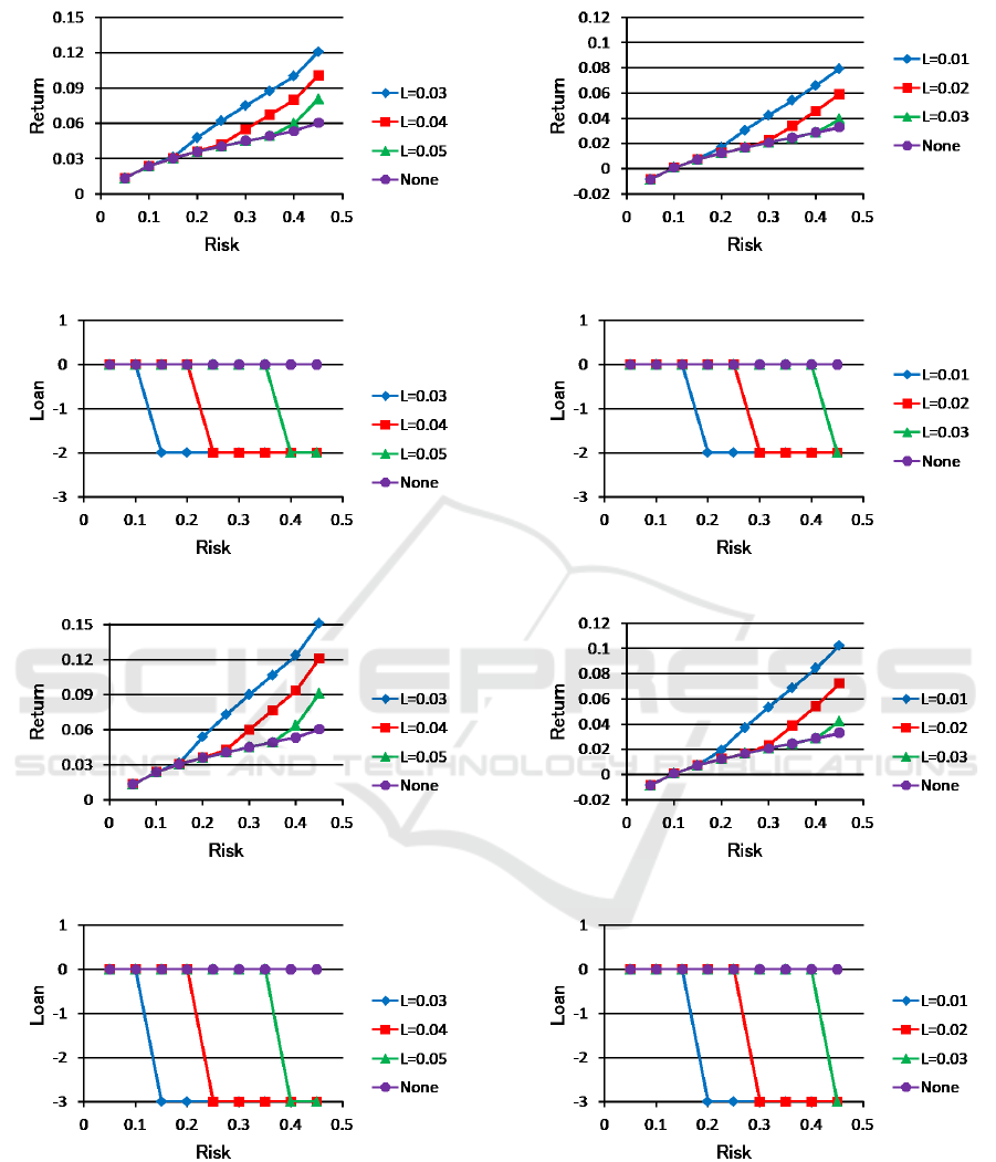
Figure 3: Efﬁcient frontier for port0 with M = 2.

Figure 4: Proportion of loan x

for port0 with M = 2.

Figure 5: Efﬁcient frontier for port0 with M = 3.

Figure 6: Proportion of loan x

for port0 with M = 3.

doesn’t use the loan, it keeps x

= 0 in Figure 4.

Figure 5 shows the efﬁcient frontier evaluated for

port0 with M = 3. Figure 6 shows the proportion of

loan x

∈ [−M, 0] for each portfolio in Figure 5.

From Figure 3 and Figure 5, we can conﬁrm that

the efﬁcient frontier is further improved by borrowing

Figure 7: Efﬁcient frontier for port1 with M = 2.

Figure 8: Proportion of loan x

for port1 with M = 2.

Figure 9: Efﬁcient frontier for port1 with M = 3.

Figure 10: Proportion of loan x

for port1 with M = 3.

much more money. Furthermore, from Figure 4 and

Figure 6, we can see that the loan is always used up

to the limit (x

= −M) regardless of its value M.

Figure 7 shows the efﬁcient frontier evaluated for

port1 with M = 2. Figure 8 shows the proportion of

loan x

∈ [−M, 0] for each portfolio in Figure 7.

An Interest Rate Decision Method for Risk-averse Portfolio Optimization using Loan

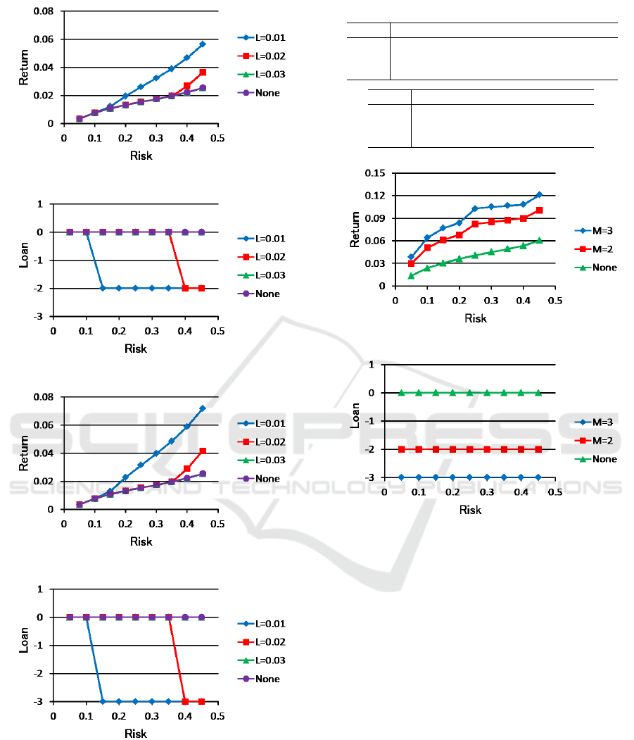
Figure 11: Efﬁcient frontier for port2 with M = 2.

Figure 12: Proportion of loan x

for port2 with M = 2.

Figure 13: Efﬁcient frontier for port2 with M = 3.

Figure 14: Proportion of loan x

for port2 with M = 3.

Figure 9 shows the efﬁcient frontier evaluated for

port1 with M = 3. Figure 10 shows the proportion of

loan x

∈ [−M, 0] for each portfolio in Figure 9.

Figure 11 shows the efﬁcient frontier evaluated for

port2 with M = 2. Figure 12 shows the proportion of

loan x

∈ [−M, 0] for each portfolio in Figure 11.

Table 4: Interest rate of loan by proposed method.

α 0.05 0.10 0.15 0.20 0.25

port0 0.005 0.010 0.015 0.020 0.020

port1 — — 0.001 0.001 0.005

port2 0.001 0.002 0.004 0.006 0.008

α 0.30 0.35 0.40 0.45

port0 0.025 0.030 0.035 0.040

port1 0.005 0.010 0.015 0.020

port2 0.010 0.010 0.012 0.015

Figure 15: Efﬁcient frontier for port0.

Figure 16: Proportion of loan x

for port0.

Figure 13 shows the efﬁcient frontier evaluated for

port2 with M = 3. Figure 14 shows the proportion of

loan x

∈ [−M, 0] for each portfolio in Figure 13.

From Figure 12 and Figure 14, the loan is not used

at all when the interest rate is high (L = 0.03).

From Figure 3 to Figure 14, we can conﬁrm that

the use of loan works well for improving the efﬁcient

frontier. Besides, the loan is always used up to the

limit as x

= −M. The lower interest rate provides

higher return and beneﬁts borrowers. On the other

hand, the high interest rate of loan doesn’t beneﬁt

lenders because such a loan is not often used. The

high interest rate of loan doesn’t beneﬁt borrowers,

either. That is because the efﬁcient frontier can’t be

improved for borrowers without using the loan.

5.3 Variable Interest Rate

From each of the data sets, POPL is formulated as

shown in (46). According to the proposed method,

COMPLEXIS 2020 - 5th International Conference on Complexity, Future Information Systems and Risk

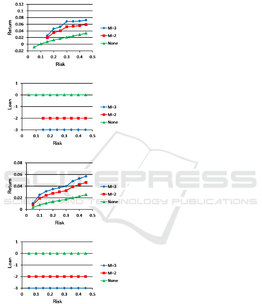
Figure 17: Efﬁcient frontier for port1.

Figure 18: Proportion of loan x

for port1.

Figure 19: Efﬁcient frontier for port2.

Figure 20: Proportion of loan x

for port2.

a proper interest rate of loan L ∈ ℜ is decided for

each of the risk α ∈ (0, 0.5) as shown in Table 4.

The loan can’t be used for port1 when the risk is too

low (α ≤ 0.1). That is because the optimal solution

⋆

∈ ℜ

of the sub-problem of POPL in (44) doesn’t

meet γ

⋆

) ≥ 0. For each pair of α and L shown in

Table 4, POPL in (46) is solved repeatedly.

Figure 15 shows the efﬁcient frontier evaluated for

port0, where the proper interest rate L ∈ ℜ in Table 4

is used for each risk α ∈(0, 0.5). Two different upper

limits, M = 2 and M = 3, are compared in Figure 15.

Figure 16 shows the proportion of loan for each

portfolio shown in Figure 15. From Figure 16, we can

conﬁrm that every portfolio except “None” borrows

money from the loan up to the limit as x

= −M.

Figure 17 shows the efﬁcient frontier evaluated for

port1 with the interest rate of loan L ∈ ℜ in Table 4.

The loan is not used for the low risks, α = 0.05 and

α = 0.1, in Figure 17. Figure 18 shows the proportion

of loan for each portfolio shown in Figure 17.

Figure 19 shows the efﬁcient frontier evaluated for

port2 with L ∈ ℜ in Table 4. Figure 20 shows the

proportion of loan for each portfolio in Figure 19.

From Figure 15 to Figure 20, we can conﬁrm that

the loan with the proper interest rate L ∈ ℜ is always

used for improving the efﬁcient frontier regardless of

the acceptable risk α ∈ (0, 0.5). Furthermore, we can

see that the return γ(x

x) of the optimal solution x

x ∈ ℜ

for POPL depends not only on the risk α but also on

the upper limit of loan M. Speciﬁcally, we can get

more return by borrowing more money.

6 CONCLUSION

Portfolio optimization using loan has been formulated

as POPL and solved in this paper. The emphasis of

our work is on the proposal of an interest rate decision

method for POPL. From an acceptable risk α, the pro-

posed method can derive a proper interest rate of loan

L that beneﬁts both borrowers and lenders. Thereby,

POPL in (24) can be also written by a rather simple

form in (46). Finally, from the result of the numeri-

cal experiment, we have conﬁrmed that the efﬁcient

frontier is improved by using the loan completely.

As mentioned above, the proposed method in this

paper beneﬁts both borrowers and lenders. Therefore,

we can expect that the proposed method contributes

to economic revitalization through active investment

using loan. On the other hand, we have to choose

the acceptable risk α ∈ (0, 0.5) carefully to use the

proposed method safely and effectively.

For future work, we will extend POPL based on a

multi-period framework. Furthermore, we would like

to include cardinality constraints into POPL.

An Interest Rate Decision Method for Risk-averse Portfolio Optimization using Loan

REFERENCES

Anagnostopoulos, K. P. and Mamanis, G. (2010). A port-

folio optimization model with three objectives and

discrete variables. Computers & Operations Re-

search, 37:1285–1297.

Angelelli, E., Mansini, R., and Speranza, M. G. (2008). A

comparison of MAD and CVaR models with real fea-

tures. Journal of Banking & Finance, 32:1188–1197.

Aranha, C. and Iba, H. (2007). Modelling cost into a ge-

netic algorithm-based portfolio optimization system

by seeding and objective sharing. In Proc. IEEE

Congress on Evolutionary Computation, pages 196–

203, Singapore.

Ash, R. B. (2008). Basic Probability Theory. Dover, Down-

ers Grove.

Beasley, J. E. (1990). OR-Library: distributing test prob-

lems by electronic mail. Journal of the Operational

Research Society, 41(11):1069–1072.

Chang, T.-J., Meade, N., Beasley, J. E., and Sharaiha,

Y. M. (2000). Heuristics for cardinality constrained

portfolio optimization. Computers & Operations Re-

search, 25:1271–1302.

Horst, R. and Pardalos, P. M. (1995). Handbook of Global

Optimization. Kluwer Academic Publishers.

Kataoka, S. (1963). Stochastic programming model.

Econometrica, 31(1/2):181–196.

Konno, H. and Yamamoto, R. (2005). Integer program-

ming approaches in mean-risk models.

Computational

Management Science, 2(4):339–351.

Konno, H. and Yamazaki, H. (1995). Mean-absolute de-

viation portfolio optimization model and its applica-

tions to Tokyo stock market. Management Science,

37(5):519–531.

opez, C. P. (2014). MATLAB Optimization Techniques.

Springer.

Mansini, R., Ogryczak, W., and Speranza, M. G. (2014).

Twenty years of linear programming based on port-

folio optimization. European Journal of Operational

Research, 234:518–535.

Markowitz, H. (1952). Portfolio selection. The Journal of

Finance, 7(1):77–91.

McCormick, G. P. (1983). Nonlinear Programming. John

Wiley & Sons.

Mokhtar, M., Shuib, A., and Mohamad, D. (2014). Mathe-

matical programming models for portfolio optimiza-

tion problem: a review. International Journal of

Mathematical and Computational Sciences, 8(2):428–

435.

Obeidat, S., Shapiro, D., and Lemay, M. (2018). Adap-

tive portfolio assets allocation optimization with deep

learning. IARIA International Journal on Advances in

Intelligent Systems, 11(1&2):25–34.

Pang, X., Zhou, Y., Wang, P., Lin, W., and Chang, V.

(2018). Stock market prediction based on deep long

short term memory neural networks. In Proc. COM-

PLEXIS 2018, pages 102–108.

Ponsich, A., Jaimes, A. L., and Coello, C. A. C. (2013).

A survey on multiobjective evolutionary algorithms

for the solution of the portfolio optimization problem

and other ﬁnance and economics applications. IEEE

Trans. on Evolutionary Computation, 17(3):321–343.

ekopa, A. (1995). Stochastic Programming. Kluwer Aca-

demic Publishers.

Price, K., Storn, R. M., and Lampinen, J. A. (2005). Dif-

ferential Evolution: A Practical Approach to Global

Optimization. Springer.

Roy, A. D. (1952). Safty ﬁrst and the holding of assets.

Econometrica, 20(3):431–449.

Rubio, F., Mestre, X., and Palomar, D. (2012). Performance

analysis and optimal selection of large minimum vari-

ance portfolios under estimation risk. IEEE Journal of

Selected Topics in Signal Processing, 6(4):337–350.

Ruppert, D. (2011). Statistics and Data Analysis for Finan-

cial Engineering. Springer.

Strumberger, I., Tuba, E., Bacanin, N., Beko, M., and Tuba,

M. (2018). Hybridized artiﬁcial bee colony algorithm

for constrained portfolio optimization problem. In

Proc. IEEE Congress on Evolutionary Computation,

pages 1–8, Rio de Janeiro, Brazil.

Tagawa, K. (2019). Group-based adaptive differential evo-

lution for chance constrained portfolio optimization

using bank deposit and bank loan. In Proc. IEEE

Congress on Evolutionary Computation

, pages 1557–

1563, Wellington, New Zealand.

Tagawa, K. (2020). Chance constrained portfolio opti-

mization using loan. In Proc. The 12th International

Conference on Information, Process, and Knowledge

Management, pages 1–6, Valencia, Spain.

Tamiz, M., Azmi, R. A., and Jones, D. F. (2013). On se-

lecting portfolio of international mutual funds using

goal programming with extended factors. European

Journal of Operation Research, 226:560–576.

COMPLEXIS 2020 - 5th International Conference on Complexity, Future Information Systems and Risk