The Bi-objective Minimum Latency Problem with Proﬁt Collection and

Uncertain Travel Times

Maria Elena Bruni

, Sara Khodaparasti

and Samuel Nucamendi-Guill

Department of Mechanical, Energy and Management Engineering, Unical, Italy

Universidad Panamericana, Facultad de Ingenier

ıa,

Alvaro del Portillo 49, Zapopan, Jalisco, 45010, Mexico

Keywords:

Minimum Latency Problem, Proﬁt, Bi-objective Optimization, Uncertainty, Risk.

Abstract:

This paper introduces a new bi-objective minimum latency problem with proﬁt collection, where routes must

be constructed in order to maximize the collected proﬁt and to minimize the total latency. These objectives

are usually conﬂicting. Thus, considering some important features, as the segmentation of the customers into

two classes, mandatory and optional, and the presence of uncertain travel times, we follow a bi-objective

approach, aiming to compute a set of Pareto-optimal alternatives with different trade-offs for a decision-maker

to choose from. In order to address this computationally challenging problem, we propose a Multi-Objective

Iterated Local Search. Computational results conﬁrm the practicality of the algorithm, in terms of the quality

of the solutions, and its computational efﬁciency in terms of time spent. We conclude that the algorithm ﬁnds

good-quality solutions for small and medium-size instances.

1 INTRODUCTION

This paper models and solves a new routing problem

of practical importance, which considers customers

with different service level agreements. The frequent

customers are mandatory to be serviced, whilst the

service requests of the non-frequent customers might

be either rejected or accepted. The attractiveness of

these additional customers relies on the potential ad-

ditional proﬁt that can be gained. A generic appli-

cation of the problem we are considering is the de-

sign of routes for technicians for repair and mainte-

nance operations. Mandatory customers are requiring

preventive maintenance operations, whereas optional

customers are requiring a repair service. In this ap-

plication, vehicles are used only for carrying material

and personnel. Thus, we can suppose that the vehi-

cle capacity is unlimited. There are other applicative

contexts in which the company has to regularly visit

customers with long-term relations, whereas potential

customers, usually located close to the existing ones,

can be serviced, in an effort to expand the existing

customer base. A similar setting is also faced by small

package shipping companies, where commercial cus-

tomers need to be regularly visited, while residential

customers are only visited on an ad hoc basis. The

aforementioned problems pose the same challenge:

designing a set of routes with the aim of visiting all

the mandatory customers and, at the same time, de-

termining the subset of the potential customers that

will be included in the routing plans. Although such

problems are frequently used to model real cases, they

are often modelled as single objective models, despite

the fact that in the majority of applications are multi-

objective in nature. Two conﬂicting objectives can be

considered relevant in our case. The ﬁrst is to max-

imize the total collected proﬁt, while the second is

to minimize the total arrival time to the customers.

Combining these conﬂicting objectives into one sin-

gle objective is questionable, since they are expressed

in different measurement units, motivating the mod-

elling of the problem as a bi-objective one.

The main contributions of this paper are:

• The introduction of the bi-objective minimum la-

tency problem with proﬁt collection, considering

realistic features such as the presence of optional

customers and stochastic travel times.

• While modeling this problem, we consider a risk-

averse measure for the total arrival time, instead

of the widely used expected risk measure.

• We present a more general and risk-averse ap-

proach, which includes the well known Condi-

tional Value at Risk (CVaR, for short) as a special

case, providing a uniﬁed framework for dealing

with risk.

Bruni, M., Khodaparasti, S. and Nucamendi-Guillén, S.

The Bi-objective Minimum Latency Problem with Proﬁt Collection and Uncertain Travel Times.

DOI: 10.5220/0009181801090118

In Proceedings of the 9th International Conference on Operations Research and Enterprise Systems (ICORES 2020), pages 109-118

ISBN: 978-989-758-396-4; ISSN: 2184-4372

109

• We design and implement an iterated greedy pro-

cedure to efﬁciently deal with instances of reason-

able size that can be used for a broad class of risk

measures.

The paper is organized as follows. The next sec-

tion is dedicated to the literature review. Section 3

presents the problem description, formalized in the

Appendix. Section 4 is devoted to the description of a

solution approach. We discuss the effectiveness of the

method and report computational results in Section 5.

We conclude in Section 6.

2 LITERATURE REVIEW

The minimum latency problem (MLP) or travelling

repairman problem (TRP) is one of the most famous

customer-centric routing problems. It consists in ﬁnd-

ing a tour starting from a depot node, which mini-

mizes the sum of the elapsed times (or latencies) to

reach a given set of nodes. The problem arises in situ-

ations in which the arrival time has a crucial role in the

customers satisfaction and it has recently attracted the

attention of the researchers, due to its importance in

applicative ﬁelds such as emergency logistics (Bruni

et al., 2018b), delivery logistics (Bruni et al., ), and

manufacturing contexts such as machine scheduling

(Bruni et al., 2019).

This problem has been extensively studied by a

large number of researchers who proposed several

exact and non-exact approaches. Lucena (Lucena,

1990) and Bianco et al. (Bianco et al., 1993) pro-

posed early exact enumerative algorithms, in which

lower bounds are derived using a Lagrangian relax-

ation. Fischetti et al. (Fischetti et al., 1993) pro-

posed an enumerative algorithm that makes use of

lower bounds obtained from a linear integer program-

ming formulation. Different mixed integer program-

ming formulations with various families of valid in-

equalities have been proposed in the last years (Bi-

gras et al., 2008; Ezzine et al., 2010; M

endez-D

ıaz

et al., 2008; Van Eijl, 1995). Salehipour et al. (Sale-

hipour et al., 2011) ﬁrst proposed a simple composite

algorithm based on a GRASP, improved with a vari-

able neighborhood search procedure. In (Mladenovi

et al., 2013a), Mladenovi

c et al. presented a general

variable neighborhood search metaheuristic enhanced

with a move evaluation procedure facilitating the up-

date of the incumbent solution. Silva et al. (Silva

et al., 2012) presented a composite multi-start meta-

heuristic approach consisting of a GRASP and a ran-

domized variable neighborhood descent algorithm. A

direct extension of the TRP/MLP is the multiple trav-

eling repairman problem (k-TRP) that considers iden-

tical vehicles. Although many researchers have stud-

ied the TRP, the literature on the multiple vehicle case

is surprisingly limited. Recently, Nucamendi-Guill

et al. (Nucamendi-Guill

en et al., 2016; Nucamendi-

Guill

en et al., 2018) presented an efﬁcient new formu-

lation, deﬁned on a multi-level network, for the deter-

ministic k-traveling repairman problem enhanced by

an iterative greedy metaheuristic. Several metaheuris-

tic algorithms have been designed for efﬁciently solv-

ing routing problems with cumulative costs and its

variants (Mladenovi

c et al., 2013b; Ngueveu et al.,

2010; Ribeiro and Laporte, 2012; Rivera et al., 2015).

The k-Traveling Repairmen Problem with Prof-

its (k-TRPP) has been introduced by Dewilde et al.

(Dewilde et al., 2013) as an extension of the TRP

where the service at each node is rewarded with a non-

negative proﬁt, which decreases with arrival time at

the node. Recently, in (Yongliang et al., 2019) a popu-

lation based hybrid evolutionary search algorithm has

been proposed for solving the problem, combining a

randomized greedy construction method for initial so-

lution generation and a dedicated variable neighbor-

hood search for local optimization. Although several

contributions have addressed uncertainty in routing

problems (Beraldi et al., 2005; Bruni et al., 2014; Be-

raldi et al., 2015a; Beraldi et al., 2015b) only a few

contributions focused on incorporating uncertainty in

the k-TRPP (Bruni et al., 2018a; Beraldi et al., 2019;

Bruni et al., 2020). Moreover, all of the aforemen-

tioned works focused on the single-objective version

of the problem, seeking for a trade-off between re-

ward and variance, two different objectives that are

not calculated with the same metric.

To the best of our knowledge, the only two

contributions dealing with the multi-objective MLP

are (Arellano-Arriaga et al., 2019; Arellano-Arriaga

et al., 2017). Both papers consider a bi-objective

approach for the MLP, considering a single-vehicle

tour and minimising the travel time (as a measure of

distance) and the latency of that tour. In this paper,

we address the problem under a risk-averse perspec-

tive considering a ﬂeet of vehicles, the proﬁts and the

presence of optional customers. To the best of out

knowledge, the the problem studied in this paper has

never been tackled before.

3 PROBLEM FORMULATION

Let consider an undirected graph G = V, E where

V = {0, 1, 2, . . . , n} corresponds to the node set and

E denotes the edge set. Node 0 denotes the depot

and V

= {1, 2, . . . , n} represents the set of customers

further partitioned into two subsets: M is the set of

ICORES 2020 - 9th International Conference on Operations Research and Enterprise Systems

110

mandatory customers, while O is the set of optional

customers. For each demand node i ∈V

, a proﬁt p

deﬁned. Additionally, there is a homogeneous ﬁxed

ﬂeet of K uncapacitated vehicles, dispatched from the

depot and that can serve any route assigned.

The aim is to design vehicle routes for serving a

mix of regular and on the spot customers, while ensur-

ing that the arrival time at the customers is minimized

and the proﬁt collected is maximized. To this end,

this paper addresses a combined minimum latency

and proﬁt maximizing repairman problem through a

bi-objective model that captures the proﬁt collecting

nature, as well as the main feature of the minimum

latency problem.

In particular, the ﬁrst objective function is the to-

tal proﬁt collected. Let assume that we have a set of

routes π

, k = 1, . . . K, then, the collected proﬁt can be

expressed as:

P =

k=1

i∈π

Now, let assume that each edge l ∈ E has an asso-

ciated random travel time

, with a given mean µ

and

variance σ

. When the travel times are considered

random, the arrival time of each vehicle at generic

node i is itself a random variable (denoted with

In particular, the arrival time at each node is the sum

of the travel times associated to the links l ∈ π

i.e.

belonging to the subpath connecting the depot to the

node i. The total arrival time, deﬁned as

T =

k=1

i∈π

is itself a random variable.

Since the decision-maker is risk-averse when

making a decision, the problem does not merely en-

tail the minimization of the expected arrival time, but

it must also consider the decision maker’s attitude

against risk.

Formally, a risk measure is a map ρ : X − > R

that attaches a scalar value to each random vari-

able X : Ω− > R , governed by a probability distri-

bution function F

, whose moment-generating func-

tion M

z = IEe

exists for all z ≥ 0. Artzner et

al. (Artzner et al., 1999) stated a set of properties

that should be desirable for any risk measure. The

four axioms they stated are: Monotonicity, Transla-

tion equivariance, Subadditivity and Positive Homo-

geneity. Given two random variables X and Y and a

risk function, ρ, we can deﬁne the properties as fol-

lows.

• Monotonicity- A risk measure is monotone, if for

all X, Y : X ≤Y ρX ≤ρY , i.e., higher losses mean

higher risk

• Translation Equivariance- A risk measure is trans-

lation equivariant, if for all X, and scalars c ∈ R:

ρX + c = ρX + c, i.e., increasing (or decreasing)

the loss increases (decreases) the risk by the same

amount

• Subadditivity- A risk measure is subadditive, if

for all X, Y ρX + Y ≤ ρX + ρY , i.e., diversiﬁca-

tion decreases risk

• Positive Homogeneity- A risk measure is posi-

tively homogeneous, if for all X , λ ≥ 0: ρλX =

λρX, i.e., doubling the size doubles the risk

Any risk measure which satisﬁes these axioms is said

to be coherent (Artzner et al., 1999).

A general class of risk measures is represented by

the spectral risk measures, ﬁrst introduced by Acerbi

(Acerbi, 2002). A spectral risk measure, denote by

SRM

is a function parameterized by φ, a nondecreas-

ing normalized right-continuous integrable probabil-

ity density function, such that φ ≥ 0, and

φpd p = 1.

The density function φ is also called an risk spectrum.

It can be deﬁned as follows:

SRM

φpF

−1

pd p =

φpVaR

d p.

Spectral risk measures satisfy the properties of mono-

tonicity, convexity, translation invariance and co-

herency. In most real-life applications, the probability

distribution of the travel times is typically unknown

and only indirectly observable through historical sam-

ples. A remedy for this difﬁculty is to adopt a distribu-

tionally robust approach, assuming that the probabil-

ity distribution is merely known to belong to an ambi-

guity set, typically deﬁned as the family F of all dis-

tributions that have known ﬁrst and second moments.

This ambiguity prompts us to investigate the quan-

tiﬁcation of the risk in this more general setting. In

this case, solutions are evaluated under the worst-case

over all the distributions in the family F and hence,

consistent with the known moments. The resulting

Worst-Case Spectral Risk Measure (WCSRM) repre-

sents a conservative (that is, pessimistic) approxima-

tion for the true (unknown) SRM. We can deﬁne the

WCSRM as follows:

WCSRM = sup

F∈F

SRM

As proposed in (Li, 2018), it can be proved that the

WCSRM admits an elegant closed form expression:

WCSRM = µ + σ

pd p −1

Considering the above deﬁnitions, the risk crite-

rion reduces to the worst-case Conditional Value at

The Bi-objective Minimum Latency Problem with Proﬁt Collection and Uncertain Travel Times

111

Risk

, when

φp =

(

1−α

if p > α

0 if p ≤ α.

and we have

pd p =

1−α

. In fact, we obtain the

well known formula

WCVaR = sup

F∈F

CVaR

= µ + σ

1 −α

A similar closed form (assuming Normal distribu-

tions) can also be obtained for another well-known

risk measure, the Entropic VaR (EVaR), recently

introduced in Ahmadi-Javid (Ahmadi-Javid, 2012a;

Ahmadi-Javid, 2012b), which is the tightest possible

upper bound for VaR and the CVaR. The EVaR of X

with conﬁdence level α is deﬁned as follows:

EVaR

= in f

z>0

{zln



−1

1 −α



} =

= in f

z>0

{zlnIE



exp





−zln1 −α}

Despite its apparent complexity, also the EVaR

can be boiled down to the following closed form ex-

pression assuming normally distributed random vari-

ables:

EVaR

= µ + σ

√

−2ln1 −α.

The above result provides a uniﬁed perspective on

solving the problem under different risk measures

with same objective function structure,

µ + Γσ

just by modifying the scale factor Γ of the standard

deviation. Applying this risk measure to the total ar-

rival time (T

risk

) leads to the following objective func-

tion (for a ﬁxed set of routes π

, k = 1, . . . K): The total

completion time, deﬁned as

risk

k=1

i∈π

+ Γ

k=1

i∈π

VAR

where VAR represents the standard deviation of the

total arrival time. The mathematical formulation of

the problem is reported in the Appendix.

Basically, CVaR is deﬁned as the average of the α%

worst cases weighted with a uniform weight. More for-

mally, the CVaR risk measure at a given conﬁdence level

α ∈0, 1, quantiﬁes the expected loss of the random variable

in the worst 1 −α% of cases Hence:

CVaR

= IEX |X ≥VaR

If F

is continuous, then we have

CVaR

1 −α

VaR

d p

4 HEURISTIC PROCEDURE

Our heuristic approach for approximating the Pareto-

front is based on three main procedures: a construc-

tive phase, an improvement phase and a perturba-

tion mechanism. The algorithm requires as input the

following sets and parameters: the number of cus-

tomers n, the number of vehicles K, the set of manda-

tory customers M and the set of optional customers

O. In our algorithm, a solution is represented by

s = {π

, π

, . . . , π

}. The pseudcode is shown in 1,

where Sm denotes the set of mandatory nodes not yet

visited, Sa the set of non-visited nodes and Sp the cur-

rent partial solution. The algorithm ends when the

maximum number of iterations (Maxiter) is reached.

Algorithm 1: Pseudo-code for the heuristic procedure.

Data: n, K

1 Initialization: s = {0}, iter := 0, MaxIter := T ,

Sa = V

, Sm = M

2 ConstructiveProcedure

3 ImprovementProcedure

4 ParetoSetInsertion

5 while iter < MaxIter do

6 PerturbationProcedure

7 ConstructiveProcedure

8 ImprovementProcedure

9 ParetoSetInsertion

10 iter ← iter + 1

11 end

12 Filter the Pareto Front (F

)

Result: F

In what follows, we will specialize each main step

of the algorithm.

4.1 Constructive Procedure

This procedure is based on the parallel route building

strategy originally proposed in (Potvin and Rousseau,

1993). The set of unrouted customers is denoted by

(Sa), the current partial solution by (Sp) the cost ma-

trix by C and the number of customers per route by

in Sp. The procedure also considers a generalized

regret criterion for the selection of the customers to

include in the solution.

For the ﬁrst iteration, the constructive procedure

starts with the empty routes in Sp. The procedure se-

lects the customers in Sa with the greatest expected

travel time with respect to the depot, giving priority

to the mandatory customers. Once all of the routes

have at least one customer, the procedure continues

by sequentially inserting the remaining customers in

Sa, always prioritizing the mandatory nodes. For this,

the cost of insertion is computed based on the general-

ized regret measure described in (Nucamendi-Guill

ICORES 2020 - 9th International Conference on Operations Research and Enterprise Systems

112

et al., 2018) but considering the risk measure associ-

ated to the latency. The procedure ends when all of

the mandatory customers have been assigned (inde-

pendently of the remaining customers in Sa). For in-

stance, if the ﬁrst Sm customers assigned correspond

to the mandatory ones, then the constructive proce-

dure ﬁnalizes the assignment (even when there are n

- Sm customers not assigned), and the solution cre-

ated goes to the improvement procedure. On the other

hand, optional nodes can be inserted before ﬁnishing

the insertion of the mandatory nodes. Figure 2 shows

the pseudocode for this procedure.

Algorithm 2: Outline of the Constructive Procedure.

Data: Sa, Sm

1 while |Sm| > 0 or |Sa| > 0 do

2 if there are empty routes then

3 Initialize them with customers i ∈ Sa that

have the highest values of π

−µ

4 Sa := Sa \i and if i ∈ M Sm := Sm \i

5 end

6 foreach customer in Sa do

7 Determine the best insertion points over

all the K partial routes

8 Compute the regret between the values of

all insertion points and the value of the

best insertion point

9 end

10 Insert the ﬁrst customer with the highest regret

into its best place in s

11 Update Sa, Sm

12 end

13 Compute the total collected proﬁt P and the total

arrival time T for the current solution s

14 return s

After the solution is improved, it is compared

against the non-dominated solutions found so far. De-

tails of the improvement phase are provided in the

next section.

4.2 Improvement Procedure

After the initial construction is obtained, the solution

is sent to a improvement procedure that applies ﬁve

different local search strategies, arranged in two ma-

jor groups: Intra route neighborhoods (Intra RN) and

inter-route neighborhoods (Inter RN). The neighbor-

hoods used are:

• Swap move: operator that exchanges the position

of two nodes, i and j, both belonging to the same

route.

• Reallocation move: operator that removes a cus-

tomer from its current position on the route and

reinserts it in a different position on the same

route.

• 2-opt move: Two adjacent edges are deleted in the

tour, then the arcs are reversed and reconnected in

a different way.

• Interchange move: Two nodes, each belonging to

a different route, exchange their respective posi-

tions (when possible with respect to the remaining

vehicles capacities).

• Insertion move: A customer is removed from its

current position in the tour and inserted in a new

position into a different route.

The intra RN includes the swap, reallocation and

2-opt moves, whereas the inter RN involves the in-

terchange and insertion moves. The intra RN starts

by executing the swap move and it goes into a loop

where the three local searches are iteratively exe-

cuted, beginning with the reallocation move. This

loop ends when none of the neighbourhoods can im-

prove the current solution in at least one objective. On

the other hand, the inter RN performs ﬁrst the inter-

change move and then the solution goes into a loop

in which the Insertion and Interchange moves are ap-

plied iteratively. Similarly, the inter RN procedure

ends when none of the neighborhoods can improve

their input solution. After ﬁnishing the improvement

procedure, the solution is evaluated to verify if it can

be candidate to be included in the Pareto Front. The

procedure of evaluation determines if the solution is

non-dominated, then it is inserted into the a list CS.

4.3 Perturbation Procedure

The perturbation procedure consists of a partial-

removal mechanism that randomly selects a group of

customers in s and assign them into Sa and the re-

maining clients in the routes are re-allocated to the

ﬁrst positions in their corresponding route preserving

the order in which they were sequenced in the selected

solution. In case the one or more customers removed

belong to the mandatory set, then the indicator Sm is

updated correspondingly.

4.4 Pareto Candidate Set Insertion

In every iteration, this mechanism evaluates if the so-

lution obtained (after ﬁnalizing the improving proce-

dure) is non-dominated with respect to the set of so-

lutions found by the algorithm and stored in the can-

didate set (CS). It is evident that, for the ﬁrst itera-

tion, the mechanism immediately includes the solu-

tion obtained. From the second to the last iteration,

the current solution is compared with the ones that

have been previously inserted in the set. If the cur-

rent solution is non-dominated then it is added, oth-

erwise, it is discarded, and a new initial solution is

The Bi-objective Minimum Latency Problem with Proﬁt Collection and Uncertain Travel Times

113

constructed. It is important to mention that, to ac-

celerate the computation time, the case for which the

current solution would dominate any of the previous

is not evaluated. As a result, the set of CS must con-

tain at most MaxIter different solutions. To ﬁnalize

the procedure of obtaining the non-dominated Pareto

set (F

), a mechanism of obtaining the ﬁnal set of non-

dominated solutions is implemented. As mentioned

above, since Pareto Candidate Set Insertion only eval-

uates if any of the previous inserted solutions domi-

nates the current solution but not vice-versa, this pro-

cedures compares all of the solutions in the set to

determine which ones belong to the non-dominated

front.

5 COMPUTATIONAL RESULTS

To evaluate the proposed approach, we modiﬁed a

set of benchmark instances originally proposed by

Augerat et al. (Augerat et al., 1995) (P-instances) and

Christoﬁdes and Elion (Christoﬁdes and Eilon, 1969)

(E-instances) and also used in (Bruni et al., 2020). In

those instances, we incorporated the information de-

noting whether a customer is mandatory to be visited

or not. We have considered the general expression

Γ =

1 −α

for the risk measure, with different value of α =

0.1, 0.5, 0.9, to model different risk aversion levels.

The algorithm was coded in C++ and the experiments

were executed using a PC Intel

Core

i7 @2.30

GHz with 16 GB of RAM Memory under Windows

10 as OS. To account for the the randomness of the

algorithm, it was ran 10 times per instance, con-

sidering different seed values at each execution and

MaxIter = 50. To evaluate the performance of the

algorithm, three quality multiobjective metrics were

used:

• Number of points on the Pareto-Front (NPF)

(Schott, 1995; Van Veldhuizen, 1999): This met-

ric determines the ability to provide more choices

for the decision-maker. The larger, the better.

• The k-nearest neighbor density estimation tech-

nique (k-D) (Zitzler et al., 2001). This metric

allows to estimate the density of the fronts. In

this work, the three density estimator is used. The

smaller, the better.

• The Hypervolume of the space covered (Zitzler

and Thiele, 1999). The main idea behind this met-

ric is to compute the area of objective function

space covered by the nondominated vectors. This

Table 1: Values of four quality metrics over E-instances (10

executions per instance) with a value of α = 0.1.

Instance

name

Average

NPF k-D Hypervolume CPU time

En22k4 17.00 0.096 0.275 0.413

En23k3 10.30 0.179 0.394 0.382

En30k3 1.80 0.000 0.000 1.426

En30k4 3.80 0.361 0.470 1.736

En33k4 8.90 0.214 0.379 2.531

En51k5 15.40 0.119 0.247 18.679

En76k7 17.30 0.111 0.297 95.412

En76k8 20.50 0.087 0.235 109.466

En76k10 17.30 0.099 0.230 137.650

En76k14 26.20 0.065 0.221 173.438

Table 2: Values of four quality metrics over E-instances (10

executions per instance) with a value of α = 0.5.

Instance

name

Average

NPF k-D Hypervolume CPU time

En22k4 18.60 0.080 0.226 0.417

En23k3 9.80 0.203 0.400 0.376

En30k3 1.50 0.000 0.000 1.415

En30k4 1.00 0.000 0.000 1.722

En33k4 8.20 0.233 0.358 2.530

En51k5 16.70 0.101 0.244 18.524

En76k7 18.10 0.098 0.293 95.498

En76k8 20.70 0.089 0.203 109.600

En76k10 18.40 0.102 0.319 137.543

En76k14 29.20 0.057 0.204 173.426

metric estimates the size of the global dominated

set in objective space. The larger, the better.

Additionally, we evaluate the elapsed CPU time

in seconds to determine the effectiveness of the algo-

rithm in ﬁnding solutions within a reasonable compu-

tational time.

Tables 1 to 6 show the average values for the pro-

posed metrics. Column 1 indicates the name of the

instance, while columns 2, 3 and 4 report the aver-

age valued for the above-mentioned metrics. The last

column reports the elapsed time measured in seconds.

Speciﬁcally, Tables 1 to 3 and 4 to 6 report the re-

sults for different values of α (0.1, 0.5 and 0.9, corre-

spondingly). The reason of considering these values

is to determine the ability of the algorithm to model

the risk aversion.

According to the information shown in Tables 1–

3, the algorithm produced dense fronts for all the val-

ues of α and good values of the hypervolume. To

graphically display the performance of the algorithm

over the group of E-instances, the ones with the mini-

mum and maximum sizes were selected (En22k4 and

En76k14, respectively) considering the front with the

maximum number of points for each value of α for

comparison. As can be observed, in both cases, the

value of α = 0.9 provides fronts with highest values of

reward (and minimum values of risk) whereas, for the

ICORES 2020 - 9th International Conference on Operations Research and Enterprise Systems

114

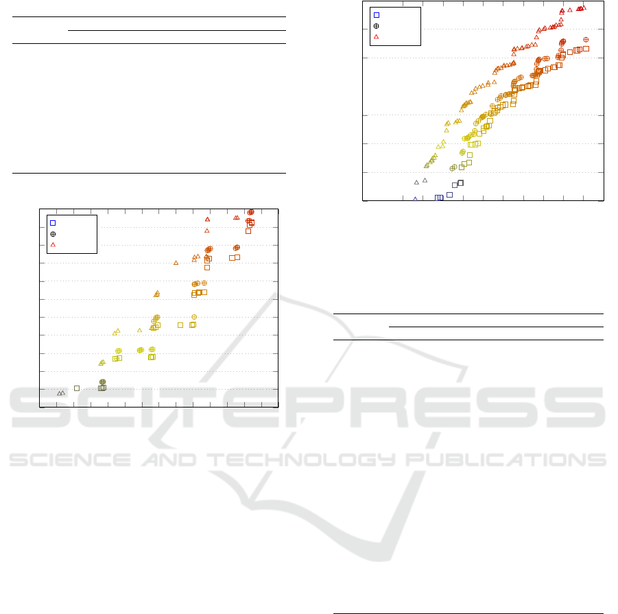
Table 3: Values of four quality metrics over E-instances (10

executions per instance) with a value of α = 0.9.

Instance

name

Average

NPF k-D Hypervolume CPU time

En22k4 15.00 0.093 0.252 0.413

En23k3 9.30 0.209 0.361 0.386

En30k3 2.70 0.577 0.634 1.441

En30k4 9.70 0.234 0.529 1.706

En33k4 8.20 0.266 0.482 2.554

En51k5 16.50 0.108 0.256 17.648

En76k7 19.60 0.093 0.298 95.793

En76k8 22.00 0.082 0.218 109.917

En76k10 17.90 0.101 0.256 137.707

En76k14 38.50 0.046 0.150 193.409

1,600

1,700

1,800

1,900

2,000

2,100

2,200

2,300

2,400

2,500

2,600

2,700

2,800

2,900

3,000

0.5

0.55

0.6

0.65

0.7

0.75

0.8

0.85

0.9

0.95

1.05

·10

Total Reward

Total Risk

alpha = 0.9

alpha = 0.5

alpha = 0.1

Figure 1: Pareto front for instance En22k4.

case when α = 0.1, the values of risk are the largest.

Thus, it can be concluded that, the parameter α has an

effect over the quality of the solutions.

Tables 4, 5 and 6 summarizes the results over the

P-instances.

For the set of P-instances, the algorithm showed

a similar behavior as for the E-instances. Regarding

the number of points, it is clear that the parameter α

has not effect. Similarly, as the size of the instance

increases, the average values of k-distances reduce,

indicating that the algorithm produces dense fronts.

With respect to the hypervolume, there is not a clear

conclusion about the quality of the results.

Figures 3 and 4 show the results obtained for in-

stances Pn16k2 and Pn76k5. As it can be noticed, for

the instance Pn16k2, all of the values of α provided

very similar Pareto fronts, which indicates that solu-

tions are not deteriorating as the value of α increases.

On the contrary, for the instance Pn76k5, the value of

α = 0.1 produced the Pareto front with smallest val-

ues of reward and high values of risk. In the case of

the hypervolume, the value of α = 0.1 produced the

smallest values in average.

2.7

2.75

2.8

2.85

2.9

2.95

3.05

3.1

3.15

3.2

·10

0.9

0.95

1.05

1.15

1.2

1.25

·10

Total Reward

Total Risk

alpha = 0.9

alpha = 0.5

alpha = 0.1

Figure 2: Pareto front for instance En76k14.

Table 4: Values of four quality metrics over P-instances (10

executions per instance) with a value of α = 0.1.

Instance

name

Average

NPF k-D Hypervolume CPU time

Pn16k8 6.3 0.401 0.744 0.251

Pn19k2 4.7 0.518 0.857 0.210

Pn20k2 3.7 0.584 0.729 0.319

Pn21k2 6.4 0.330 0.578 0.348

Pn22k2 9.9 0.188 0.654 0.440

Pn23k8 12.4 0.154 0.764 1.794

Pn40k5 9.6 0.173 0.577 14.022

Pn45k5 12.4 0.150 0.750 24.161

Pn50k7 19.3 0.090 0.766 25.448

Pn50k8 9.9 0.160 0.646 26.636

Pn50k10 12.4 0.130 0.647 57.349

Pn51k10 12.5 0.125 0.772 35.037

Pn55k7 13.8 0.125 0.734 33.569

Pn55k8 12.3 0.156 0.796 37.299

Pn55k10 16.8 0.101 0.624 54.669

Pn60k10 19.6 0.087 0.754 65.975

Pn60k15 17 0.042 0.268 94.188

Pn65k10 23.3 0.046 0.265 93.541

Pn70k10 15.5 0.099 0.559 244.324

Pn76k4 9.5 0.173 0.614 80.482

Pn76k5 32.2 0.052 0.837 96.904

Regarding the CPU time, the algorithm showed a

consistent performance over the E- and P-instances

(increasing the execution time as the size of the in-

stance increases).

6 CONCLUSIONS

In this work, we study a novel minimum latency bi-

objective problem with proﬁt collection and optional

customers. For this problem a heuristic approach was

proposed and developed for a broad class of risk mea-

sures. The performance was assessed using a set of

The Bi-objective Minimum Latency Problem with Proﬁt Collection and Uncertain Travel Times

115

Table 5: Values of four quality metrics over P-instances (10

executions per instance) with a value of α = 0.5.

Instance

name

Average

NPF k-D Hypervolume CPU time

Pn16k8 6.3 0.392 0.734 0.245

Pn19k2 4.4 0.653 0.994 0.209

Pn20k2 4 0.651 0.592 0.312

Pn21k2 6.1 0.309 0.671 0.346

Pn22k2 10.6 0.182 0.692 0.458

Pn23k8 12.1 0.167 0.859 1.770

Pn40k5 10.4 0.168 0.693 13.772

Pn45k5 13.1 0.137 0.631 24.801

Pn50k7 21.6 0.070 0.616 26.879

Pn50k8 11 0.168 0.784 29.604

Pn50k10 11.4 0.139 0.710 56.368

Pn51k10 11.3 0.157 0.770 35.650

Pn55k7 13.1 0.148 0.796 34.495

Pn55k8 12.7 0.154 0.793 37.371

Pn55k10 16.1 0.115 0.677 54.255

Pn60k10 20.8 0.076 0.672 66.105

Pn65k10 20.9 0.055 0.342 93.630

Pn70k10 16.5 0.102 0.637 188.625

Pn76k4 12.3 0.143 0.835 82.182

Pn76k5 35.6 0.051 0.896 95.832

Table 6: Values of four quality metrics over P-instances (10

executions per instance) with a value of α = 0.9.

Instance

name

Average

NPF k-D Hypervolume CPU time

Pn16k8 7.5 0.324 0.775 0.237

Pn19k2 4.1 0.619 0.836 0.205

Pn20k2 3.3 0.715 0.688 0.325

Pn21k2 6.5 0.289 0.522 0.358

Pn22k2 12.6 0.162 0.811 0.433

Pn23k8 12.6 0.147 0.706 1.786

Pn40k5 10.2 0.184 0.655 13.765

Pn45k5 14.2 0.129 0.791 24.142

Pn50k7 21.1 0.083 0.790 26.536

Pn50k8 12.3 0.132 0.784 29.412

Pn50k10 12 0.141 0.733 56.085

Pn51k10 12.2 0.143 0.769 35.643

Pn55k7 13.7 0.124 0.798 33.561

Pn55k8 15.1 0.117 0.772 37.396

Pn55k10 19.4 0.088 0.716 56.543

Pn60k10 22.9 0.054 0.295 66.403

Pn60k15 1 – – 93.891

Pn65k10 22.4 0.072 0.743 94.151

Pn70k10 18 0.094 0.633 188.721

Pn76k4 9.9 0.181 0.738 84.142

Pn76k5 34.4 0.050 0.852 95.949

benchmark instances that were properly adjusted to

analyze this particular problem. Speciﬁcally, the val-

ues of the multiobjective metrics indicate that the al-

gorithm is able to ﬁnd good quality fronts in a com-

petitive computational time. The algorithm makes a

positive contribution towards ﬁnding a trade-off be-

tween the proﬁt and the risk aversion.

Future work can include the analysis of the case

of capacitated vehicles or the inclusion of an objec-

tive function which is able to balance the maximum

traveled distance among different vehicles, to provide

equity in labor shifts. The incorporation of parame-

700

750

800

850

900

950

1,000

600

700

800

900

1,000

1,100

1,200

1,300

1,400

1,500

Total Reward

Total Risk

alpha = 0.9

alpha = 0.5

alpha = 0.1

Figure 3: Pareto front for instance Pn16k8.

2.7

2.8

2.9

3.1

3.2

3.3

·10

1.15

1.2

1.25

1.3

1.35

1.4

1.45

1.5

·10

Total Reward

Total Risk

alpha = 0.9

alpha = 0.5

alpha = 0.1

Figure 4: Pareto front for instance Pn76k5.

ters such as time windows, or due dates for each node

may also help to model real-life situations. In addi-

tion, including more objectives, mainly those related

to environmental or social goals is an interesting re-

search avenue.

ACKNOWLEDGEMENTS

This work was partially supported by the Universidad

Panamericana through the grant ”Fondo Fomento a la

Investigaci

on UP 2019”, under project code UP-CI-

2019-ING-GDL-08.

REFERENCES

Acerbi, C. (2002). Spectral measures of risk: A coherent

representation of subjective risk aversion. Journal of

Banking & Finance, 26(7):1505 – 1518.

ICORES 2020 - 9th International Conference on Operations Research and Enterprise Systems

116

Ahmadi-Javid, A. (2012a). Addendum to: Entropic value-

at-risk: A new coherent risk measure. J. Optimization

Theory and Applications, 155(3):1124–1128.

Ahmadi-Javid, A. (2012b). Entropic value-at-risk: A new

coherent risk measure. J. Optimization Theory and

Applications, 155(3):1105–1123.

Arellano-Arriaga, N., Alvarez-Socarras, A., and Martinez-

Salazar, I. (2017). A sustainable bi-objective approach

for the minimum latency problem. In Alba E., Chi-

cano F., Luque G. (eds) Smart Cities. Lecture Notes in

Computer Science.

Arellano-Arriaga, N., Molina, J., and Schaeffer, S. e. a.

(2019). A two-phase metaheuristic for the cumula-

tive capacitated vehicle routing problem. J Heuristics,

25(3):431–454.

Artzner, P., Delbaen, F., Eber, J.-M., and Heath, D. (1999).

Coherent measures of risk. Mathematical Finance,

9(3):203–228.

Augerat, P., Belenguer, J., Benavent, E., Corber

an, A., Nad-

def, D., and Rinaldi, G. (1995). Computational results

with a branch and cut code for the capacitated vehi-

cle routing problem research report 949-m. Universite

Joseph Fourier, Grenoble, France.

Beraldi, P., Bruni, M. E., Lagan

a, D., and Musmanno, R.

(2015a). The mixed capacitated general routing prob-

lem under uncertainty. European Journal of Opera-

tional Research, 240(2):382–392.

Beraldi, P., Bruni, M. E., Lagan

a, D., and Musmanno, R.

(2019). The risk-averse traveling repairman problem

with proﬁts. Soft Computing, 23(9):2979–2993.

Beraldi, P., Bruni, M. E., Manerba, D., and Mansini, R.

(2015b). A stochastic programming approach for the

traveling purchaser problem. IMA Journal of Manage-

ment Mathematics, 28(1):41–63.

Beraldi, P., Ghiani, G., Laporte, G., and Musmanno, R.

(2005). Efﬁcient neighborhood search for the proba-

bilistic pickup and delivery travelling salesman prob-

lem. Networks: An International Journal, 45(4):195–

198.

Bianco, L., Mingozzi, A., and Ricciardelli, S. (1993). The

traveling salesman problem with cumulative costs.

Networks, 23(2):81–91.

Bigras, L.-P., Gamache, M., and Savard, G. (2008). The

time-dependent traveling salesman problem and sin-

gle machine scheduling problems with sequence de-

pendent setup times. Discrete Optimization, 5(4):685–

699.

Bruni, M., Beraldi, P., and Khodaparasti, S. (2018a). A

heuristic approach for the k-traveling repairman prob-

lem with proﬁts under uncertainty. Electronic Notes

in Discrete Mathematics, 69:221–228.

Bruni, M., Forte, M., Scarlato, A., and Beraldi, P. The

traveling repairman problem app for mobile phones:

a case on perishable product delivery. AIRO Springer

Series Volume ”Advances in Optimization and Deci-

sion Science for Society, Services and Enterprises”.

Bruni, M., Khodaparasti, S., and Beraldi, P. (2019). A se-

lective scheduling problem with sequence-dependent

setup times: A risk-averse approach. pages 1–7.

SciTePress.

Bruni, M. E., Beraldi, P., and Khodaparasti, S. (2018b). A

fast heuristic for routing in post-disaster humanitar-

ian relief logistics. Transportation research procedia,

30:304–313.

Bruni, M. E., Beraldi, P., and Khodaparasti, S. (2020). A

hybrid reactive grasp heuristic for the risk-averse k-

traveling repairman problem with proﬁts. Computers

& Operations Research, 115:104–854.

Bruni, M. E., Guerriero, F., and Beraldi, P. (2014). De-

signing robust routes for demand-responsive transport

systems. Transportation research part E: logistics and

transportation review, 70:1–16.

Christoﬁdes, N. and Eilon, S. (1969). An algorithm for the

vehicle-dispatching problem. Journal of the Opera-

tional Research Society, 20(3):309–318.

Dewilde, T., Cattrysse, D., Coene, S., Spieksma, F. C., and

Vansteenwegen, P. (2013). Heuristics for the traveling

repairman problem with proﬁts. Computers & Opera-

tions Research, 40(7):1700–1707.

Ezzine, I. O., Semet, F., and Chabchoub, H. (2010). New

formulations for the traveling repairman problem. In

Proceedings of the 8th International conference of

modeling and simulation. Citeseer.

Fischetti, M., Laporte, G., and Martello, S. (1993). The

delivery man problem and cumulative matroids. Op-

erations Research, 41(6):1055–1064.

Li, J. Y.-M. (2018). Technical note—closed-form solutions

for worst-case law invariant risk measures with appli-

cation to robust portfolio optimization. Operations

Research, 66(6):1533–1541.

Lucena, A. (1990). Time-dependent traveling salesman

problem–the deliveryman case. Networks, 20(6):753–

763.

endez-D

ıaz, I., Zabala, P., and Lucena, A. (2008). A

new formulation for the traveling deliveryman prob-

lem. Discrete applied mathematics, 156(17):3223–

3237.

Mladenovi

c, N., Uro

sevi

c, D., and Hanaﬁ, S. (2013a). Vari-

able neighborhood search for the travelling delivery-

man problem. 4OR, 11(1):57–73.

Mladenovi

c, N., Uro

sevi

c, D., and Hanaﬁ, S. (2013b). Vari-

able neighborhood search for the travelling delivery-

man problem. 4OR, 11(1):57–73.

Ngueveu, S. U., Prins, C., and Calvo, R. W. (2010). An

effective memetic algorithm for the cumulative capac-

itated vehicle routing problem. Computers & Opera-

tions Research, 37(11):1877–1885.

Nucamendi-Guill

en, S., Angel-Bello, F., Mart

ınez-Salazar,

I., and Cordero-Franco, A. E. (2018). The cumula-

tive capacitated vehicle routing problem: New formu-

lations and iterated greedy algorithms. Expert Systems

with Applications, 113:315–327.

Nucamendi-Guill

en, S., Mart

ınez-Salazar, I., Angel-Bello,

F., and Moreno-Vega, J. M. (2016). A mixed integer

formulation and an efﬁcient metaheuristic procedure

for the k-travelling repairmen problem. Journal of the

Operational Research Society, 67(8):1121–1134.

Potvin, J.-Y. and Rousseau, J.-M. (1993). A parallel

route building algorithm for the vehicle routing and

scheduling problem with time windows. European

Journal of Operational Research, 66(3):331–340.

Ribeiro, G. M. and Laporte, G. (2012). An adaptive large

neighborhood search heuristic for the cumulative ca-

The Bi-objective Minimum Latency Problem with Proﬁt Collection and Uncertain Travel Times

117

pacitated vehicle routing problem. Computers & op-

erations research, 39(3):728–735.

Rivera, J. C., Afsar, H. M., and Prins, C. (2015). A multi-

start iterated local search for the multitrip cumulative

capacitated vehicle routing problem. Computational

Optimization and Applications, 61(1):159–187.

Salehipour, A., S

orensen, K., Goos, P., and Br

aysy, O.

(2011). Efﬁcient grasp+ vnd and grasp+ vns meta-

heuristics for the traveling repairman problem. 4or,

9(2):189–209.

Schott, J. R. (1995). Fault tolerant design using single and

multicriteria genetic algorithm optimization. Techni-

cal report, AIR FORCE INST OF TECH WRIGHT-

PATTERSON AFB OH.

Silva, M. M., Subramanian, A., Vidal, T., and Ochi, L. S.

(2012). A simple and effective metaheuristic for the

minimum latency problem. European Journal of Op-

erational Research, 221(3):513–520.

Van Eijl, C. (1995). A polyhedral approach to the delivery

man problem. Department of Math. and Computing

Science, University of Technology.

Van Veldhuizen, D. A. (1999). Multiobjective evolutionary

algorithms: classiﬁcations, analyses, and new innova-

tions. Technical report, AIR FORCE INST OF TECH

WRIGHT-PATTERSONAFB OH SCHOOL OF EN-

GINEERING.

Yongliang, L., Jin-Kao, H., and Qinghua, W. (June 2019).

Hybrid evolutionary search for the traveling repair-

man problem with proﬁts. Information Sciences.

Zitzler, E., Laumanns, M., and Thiele, L. (2001). Spea2:

Improving the strength pareto evolutionary algorithm.

TIK-report, 103.

Zitzler, E. and Thiele, L. (1999). Multiobjective evolu-

tionary algorithms: a comparative case study and the

strength pareto approach. IEEE transactions on Evo-

lutionary Computation, 3(4):257–271.

APPENDIX

In order to formulate the problem, we present

the multi-layer network proposed in the deter-

ministic context (Nucamendi-Guill

en et al., 2018;

Nucamendi-Guill

en et al., 2016), and successfully ex-

tended by (Bruni et al., 2018a) for the risk-averse vari-

ant. Let L be the set of levels L = {1, ··· , r, ··· , N},

where N = n −k + 1, and each level includes a copy

of all the customers amended also with the depot in

levels from 2 to n. Each tour in the network is repre-

sented by a path that ends in the ﬁrst level and starts

in a copy of the depot in some level. In fact, the level

number represents the position of the customer in the

tour: the customer in the ﬁrst level is the last in the

tour, the customer in the second level is the last but

one, and so on. Two distinct tours cannot visit the

same customer, neither in the same level nor in dif-

ferent levels. The model variables are deﬁned as fol-

lows. Let x

be a binary variable that takes value 1 iff

customer i is visited at level r (i.e. there are r −1 cus-

tomers to be visited after in the same tour); otherwise,

it is set to 0. If x

= 1, we say that customer i is active

at level r. Let y

i j

be another binary variable that is set

to 1 iff edge (i, j) is used to link customer i active at

level r + 1 with customer j active at level r; otherwise,

it takes value 0.

The mathematical formulation is expressed as fol-

lows.

Max : z



j∈V

r=1

0 j

i∈V

j∈V

j,i

N−1

r=1

i j



(1)

Min : z



j∈V

r=1

rµ

0 j

i∈V

j∈V

j,i

N−1

r=1

rµ

i j



−

j∈V

r=1

0 j

i∈V

j∈V

j,i

N−1

r=1

i j

(2)

r=1

≤ 1 i ∈ M (3)

r=1

= 1 i ∈ O (4)

i∈V

= K (5)

r=1

j∈V

0 j

= K (6)

= x

i ∈V

(7)

j∈V

j,i

i j

= x

r+1

i ∈V

, r = 1, 2, . . . , N −1 (8)

0 j

i∈V

i, j

i j

= x

j ∈V

, r = 1, 2, . . . , N −1 (9)

∈ {0, 1} i ∈V

, r = 1, 2, . . . , N (10)

0 j

∈ {0, 1} j ∈V

, r = 1, 2, . . . , N (11)

i j

∈ {0, 1} i, j ∈V

, i , j, r = 1, 2, . . . , N −1 (12)

The objective function z

in (1) maximizes the total

revenue.The second objective function minimizes the

risk associated with the given routes. In particular,

following the general expression discussed in Section

3, it is evaluated as the sum of the expected arrival

time at the nodes plus the standard deviation of the

total arrival time multiplied by a parameter Γ. Both

the terms can be derived by applying the standard for-

mula of the expected value and variance of the sum

of independent random variables. Constraints (3) en-

sure that the optional customers i are served at most

once. Constraints (4) guarantee that the mandatory

customers are served. Constraints (5) and (6) ensure

that only K starting and ending edges are created,

whereas constraints (7) - (9) satisfy connectivity re-

quirements. Finally, constraints (10) – (11) show the

nature of variables.

ICORES 2020 - 9th International Conference on Operations Research and Enterprise Systems

118