A Production Model with Continuous Demand for Imperfect Finished
Items Resulting from the Quality of Raw Material
Abdul-Nasser El-Kassar, Manal Yunis and Mohammad Nasr El Dine
Information Technology & Operations Management Department, Lebanese American University, Lebanon
Keywords: Inventory, Economic Order Quantity, Economic Production Quantity, Quality, Imperfect Quality, Raw
Material Inventory, Continuous Demand for Imperfect Quality.
Abstract: The purpose of this paper is to present a production process in which the quality of a single type of raw
material used to produce the finished product is considered. The common modeling approach followed by
previous research is based on discarding the imperfect quality items of raw material. In this paper, we consider
the case where both perfect and imperfect quality items of raw are used in the production process resulting in
two types of qualiy of the finished product. It is assumed that both perfect and imperfect quality items of the
finished product have continuous demand. This modeling approach has yet to be deployed. Two models that
depend on the length inventory cycle of each type of the finished product are developed. Numerical examples
are provided to illustrate the determination of the optimal production quantity. Theoretical and practical
implications are discussed, and recommendations are presented.
1 INTRODUCTION
Production control and inventory management are
two important business functions with the objective
of controlling the materials used in manufacturing
and trading. The importance of these functions lies in
the fact that keeping the right amount of inventory
with a good quality level will help organizations
avoid excess inventory and shortages, while
satisfying customers’ demand. This is crucial in an
era of globalization, where customer demand for
products has been increasing, and where
organizations should have the agility required to
respond to different demand preferences sufficiently
and on time.
In these two functions, the two models, economic
production quantity (EPQ) and the economic order
quantity (EOQ), are used to identify the optimal
quantities to order or produce to meet the demand for
a certain product.
The EOQ and EPQ models are simple to apply
and built on a number of simplifying assumptions.
For instance, the classical EPQ model ignores the cost
and quality of raw material used in the production
process. Also, the classical EPQ model views the
manufacturing process as failure free, implying that
items produced have perfect quality. This contrasts
with real life production environment, where
defective items are generated due to defective raw
materials or defective production processes (Pal et al,
2016). This study concurs with this view, and argues
that the inventory and production policy guided by
the conventional EPQ model is inappropriate as it
does not reflect what usually happens in production
processes.
Several researchers addressed this unreliable
assumption. Recently, a number of research studies
have worked on EPQ/EOQ models, taking imperfect
quality raw materials or imperfect product items into
consideration. This research direction was initiated by
Salameh and Jaber (2000), who developed an EPQ
model that counted for the imperfect items delivered
by a supplier with a known probability density
function.
Moreover, several recent studies have considered
the effects of the quality of the raw material used in
the production process (El-Kassar et al., 2012;
Yassine 2016; Yassine & AlSagheer, 2017; Yassine et
al., 2018; Yassine & El-Rabih, 2019). Yassine (2018)
presented a sustainable EPQ model with quality. In
fact, corporations have been engaging in responsible
and environmentally friendly activities that enhance
performance (El-Kassar & Singh, 2019; Singh et al.,
2019, El-Khalil & El-Kassar, 2018; El-Khalil & El-
Kassar, 2016). Such activities have been shown to lead
to other positive outcomes such as higher level of
El-Kassar, A., Yunis, M. and El Dine, M.
A Production Model with Continuous Demand for Imperfect Finished Items Resulting from the Quality of Raw Material.
DOI: 10.5220/0009181702630269
In Proceedings of the 9th International Conference on Operations Research and Enterprise Systems (ICORES 2020), pages 263-269
ISBN: 978-989-758-396-4; ISSN: 2184-4372
Copyright
c
 2022 by SCITEPRESS – Science and Technology Publications, Lda. All rights reserved
263

corporate governance (ElGammal et al., 2018) and
favorable employee attitude and behavior (El-Kassar
et al. 2017). Firms are also employing information and
communication technologies and innovation to
improve their competitiveness level (Singh et al.,
2019; Balozian et al., 2019; Yunis et al., 2018;
Balozian & Leidner, 2017; Yunis et al., 2017).
Recently, these factors have been incorporated into the
classical EPQ model (Lamba et al., 2019; Yassine,
2018).
Salameh and El-Kassar (2007) extended the EPQ
model to account for the raw material used in
production. Chan et al. (2003) presented an EPQ
model where the imperfect products are reworked or
rejected. El-Kassar (2009) presented an EOQ model
with quality in which the imperfect items have a
continuous demand for both perfect and imperfect
quality items. In other directions, several studies
considered a supply chain approach was considered
(Khan et al., 2011; Khan & Jaber, 2011; Bandaly et
al. 2014; Bandaly et al. 2016), while Bandaly &
Hassan (2019) considered an integrated production
and inventory taking into consideration deterioration
and limited storage capacity.
This research paper examines an EPQ model that
takes into consideration the situation where a single
type of raw material with a percentage of imperfect
items is all used in a production process. This EPQ
model is material-dependent and hence will yield
finished products with a proportion being defective.
The model assumes continuous demand for both the
good quality and the defective products, making it
essential to incorporate both product types in the
production model. Two models that depend on the
inventory cycle length of each type of finished
product are presented. The remaining of this paper is
organized as follows. Section 2 presents a review of
related work. The mathematical model is developed
in section 3. A numerical example is given in section
4 to illustrate the proposed model. Finally, section 5
presents a conclusion and future research
recommendations.
2 MATHEMATICAL MODEL
Consider the case where items of raw material
received from a supplier are of perfect and imperfect
quality. Both types are used in the production process
resulting in perfect and imperfect finished products.
It is assumed that both types of finished product have
continuous demand.
2.1 Notation
The following notation is used for this model are:
− Q: Number of units per order (units)
− Q*: Optimal number of units per order (units)
− D
p
: Demand rate for perfect finished products
(units/unit time)
− D
i
: Demand rate for imperfect finished products
(units/unit time)
− D: Demand rate (units/unit time): D
p
+D
i
− C: Purchasing cost per unit ($/unit)
− C
p
: Unit production cost ($/unit)
− K
o
: Ordering cost of raw material ($)
− K
s
: Set-up cost of production ($)
− C
s
: Unit screening cost ($/unit)
− C
hr
: Holding cost of raw material ($/unit/unit
time)
− C
hf
: Holding cost of finished products
($/unit/unit time)
− q: Percentage of perfect quality of raw material
− S
p
: Selling price of perfect quality products ($)
− S
i
: Selling price of imperfect quality products ($)
− S
d
: Discounted selling price of imperfect quality
products ($)
− T: Inventory cycle length (unit time) = Q/D
− T
p
: Perfect items inventory cycle (unit time)
− T
i
: Imperfect items inventory cycle (unit time)
− X: Screening rate (unit/unit time)
− P
p
: Production rate of perfect products (units/
unit time)
− P
i
: Production rate of imperfect products (units/
unit time)
− P: Production rate (units/ unit time) = P
p
+P
i
− T
s
: Screening time (unit time) = Q/X
− T
pr
: Production period (unit time) = Q/P
The decision variable is the order quantity Q and the
aim is to determine the optimal order quantity Q* that
maximizes the total profit per unit time function.
2.2 The Case Tp ≤ Ti
The objective of this model is to find the optimal
number of units per order Q* that maximizes the
expected value of the total profit per unit time
function.
Figures 1a and 1b depict the inventory levels of
raw material and the finished goods. The raw material
are screened for imperfect quality items. The
percentage q of perfect quality raw material is a
random variable having a known probability
distribution with an expected value of E[q]. After
screening, the perfect quality items of raw material
ICORES 2020 - 9th International Conference on Operations Research and Enterprise Systems
264

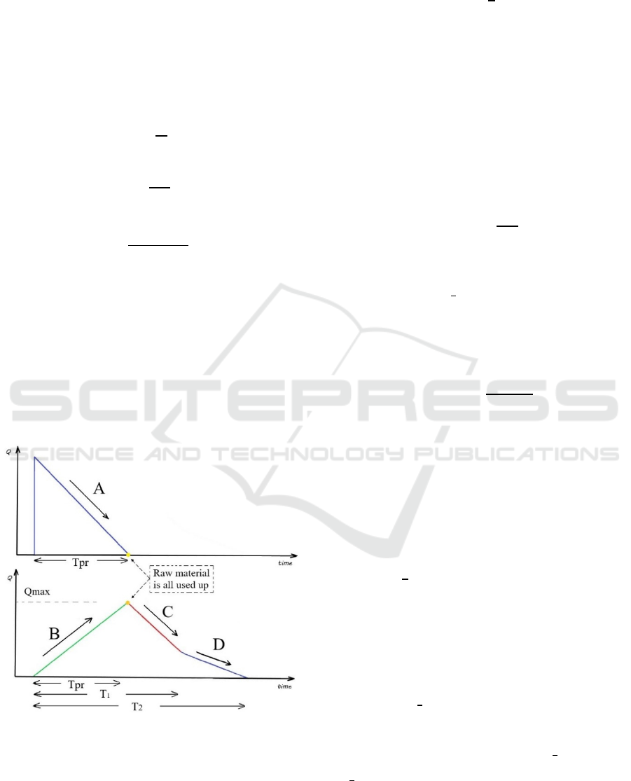
are used to produce qQ perfect quality finished items.
The remaining imperfect quality items of raw
material are also used in the production process
resulting in (1-q)Q imperfect quality finished items.
A linear relationship in the production of the two
types of items is assumed.
The combined production period as well as the
inventory cycle for the perfect and imperfect finished
items are:
T
pr
=
Q
P
(1)
T
p
=
qQ
𝐷

(2)
T
i
=
(1 − q)Q
𝐷

(3)
Let T
1
= min{T
p
, T
i
} and let T
2
= max{T
p
, T
i
}.
Assuming that T
p
> T
i
, we have T
1
= T
i
and T
2
= T
p
.
The total cost per cycle function, TC(Q),
comprises the following costs: Ordering cost, Set-up
cost, Purchasing cost, Production cost, Cost of
holding raw material, Cost of holding finished
products, and Screening cost. Hence,
TC(Q) = K
o
+ K
s
+ CQ + C
p
Q + C
s
Q + C
hr
× (Area
under curve of figure 1a) + C
hf
× (Area under curve
of figure 1b).
Figure 1a: Raw material inventory (top) Figure 2b: Finished
product inventory (bottom) Tp ≥ Ti.
First, we determine the area under curve of figure 1a.
It is worth noting that the inventory level of the raw
material is used at the production rate P. Hence, the
slope A = -P.
The area under curve of figure 1a is given by:
A
triangle
=
1
2
T

𝑄
To find the area under curve of figure 1b, we note that
during the production period, finished items are
produced at a rate of P and consumed at a rate of D =
D
p
+ D
i
. To avoid shortages, it is assumed that P > D.
Thus, finished product inventory is accumulated
at a rate of P
− (D
p
+D
i
) until a maximum inventory
level Q
max
is reached the end of the production period.
Hence, the slope B = P
− (D
p
+D
i
) and
Qmax = T
pr
[P − (D
p
+D
i
)].
First the arear under the green curve is determined as
follows:
A
triangle
=
b×h
2
where b = T
pr,
h = Qmax, and the slope of the
hypotenuse is P
− (D
p
+D
i
). Hence,
A
triangle
=
1
2
Tpr
2
[P − (D
p
+D
i
)]
Next, the area under the red curve is determined as
follows. Note that, at the end of the production period
and until time T
1
, the finished items inventory is
depleted at a rate of
− D = − (D
p
+D
i
). Hence,
A
trapezoid
=
(b
1
+b
2
)×h
2
b
1
= T
pr
[P − (D
p
+D
i
)]
h = T
1
− T
pr
But the slope of the hypotenuse is C = -(D
p
+D
i
) so
that the equation of that line would be:
Q = -(D
p
+D
i
)t + Q
o.
At t =T
pr
, Q = Qmax = T
pr
[P − (D
p
+D
i
)]. Hence,
T
pr
[P − (D
p
+D
i
)] = -(D
p
+D
i
) T
pr
+ Q
o
Thus Q
o
= T
pr
P, and hence Q = -(D
p
+D
i
) t + T
pr
P.
When t = T
1
, Q = -(D
p
+D
i
) T
1
+ T
pr
P. Thus,
A
trapezoid
=


(T
pr
(P−(D
p
+D
i
)) + T
pr
P −(D
p
+D
i
)T
1
)
(T
1
− T
pr
)
Finally, the area under the blue curve is calculated.
Note that from time T
1
until the end of the inventory
period, at time T
2
, only perfect quality finished items
are left in inventory. These items are depleted at a rate
−D
p
so that the slope is −D
p
. Thus,
A
triangle
=
1
2
(T
pr
P − (D
p
+D
i
) T
1
)(T
2
− T
1
).
Therefore,
TC(Q) = K
o
+ K
s
+ CQ + C
p
Q + C
s
Q +
1
2
C
hr
× (T
pr
Q)
+
1
2
C
hf
× T


(P  (D

+D

) + T

[P  (D

+
D

)] + T

P  T

(D

+D

)( T

 T

) +
T

P  T

(D

+D

)( T

 T

) (4)
A Production Model with Continuous Demand for Imperfect Finished Items Resulting from the Quality of Raw Material
265

Since T
p
> T
i
, T
1
= min{T
p
, T
i
}=T
i
and T
2
=
max{T
p
,T
i
} = T
p
. Substituting T
pr
=
Q
P
, T
1
= T
i
=
(1q)Q


, and T
2
= T
p
=
qQ


, the TC(Q) function
becomes:
TC(Q) = K
o
+ K
s
+ CQ + C
p
Q + C
s
Q +
1
2
C
hr
×

Q
2
P

+
1
2
C
hf
×

Q
P

2
P  (D
p
+D
i
) +


Q
P

[P
 (D
p
+D
i
)] + Q 

(1-q)Q
D
i

(D
p
+D
i
)

(1-q)Q
D
i

Q
P

+

Q


(1-q)Q
D
i

(D
p
+D
i
)


qQ
D
p

(1-q)Q
D
i
 (5)
After simplification, we have:
TC(Q) = K
o
+ K
s
+ CQ + C
p
Q + C
s
Q +
1
2
C
hr
× 
Q
2
P

+
1
2
C
hf
× 
Q
2
D
i
−
qQ
2
D
i
−
Q
2
P
+
qQ
2
D
p
−

D
p
+D
i

qQ
2
D
p
D
i
+

D
p
+D
i

q
2
Q
2
D
p
D
i
 (6)
Next, the total revenue and total profit for this model
are:
TR(Q) = S
p
qQ + S
i
(1−q)Q
TP(Q)=S
p
qQ+S
i
(1−q)Q −

K
o
+ K
s
+ CQ + C
p
Q + C
s
Q +
1
2
C
hr
×

Q
2
P

+
1
2
C
hf
×

Q
2
D
i
−
qQ
2
D
p
−
Q
2
P
+
qQ
2
D
p
−

D
p
+D
i

qQ
2
D
p
D
i
+

D
p
+D
i

q
2
Q
2
D
p
D
i


(7)
The expected value of TP(Q) is
E[TP(Q)] = S
p
Q ∙ E[q] + S
i
Q ∙ E[1−q] − K
o
−K
s
− CQ − C
p
Q − C
s
Q −
1
2
C
hr
× 
Q
2
P
−
1
2
C
hf
× 
Q
2
D
i
−
Q
2
P
 −
1
2
C
hf
× 
Q
2
D
p
−
Q
2
D
i
−

D
p
+D
i

Q
2
D
p
D
i
∙
E[q] −
1
2
C
hf
× 

D
p
+D
i

Q
2
D
p
D
i
∙ E[q
2
]
Applying the renewal reward theorem, E[TPU(Q)] =
[()]
[]
, where T= T
p
=
qQ


. Hence,
E[TPU(Q)] =
S
p
Q ∙ E[q] + S
i
Q ∙ E[1-q] - K
o
-K
s
- CQ - C
p
Q - C
s
Q -
1
2
C
hr
× 
Q
2
P

-
1
2
C
hf
× 
Q
2
D
i
-
Q
2
P
 -
1
2
C
hf
× 
Q
2
D
p
-
Q
2
D
i
-
D
p
+D
i
Q
2
D
p
D
i
× E[q]
-
1
2
C
hf
× 
D
p
+D
i
Q
2
D
p
D
i
∙ E[q
2
]
Q
D
p
∙ E[q]
Setting the derivative of the above expression equal
to zero and solving for Q, we get:
Q*=

K
o
+K
s
1
2
C
hr
×
1
P
 +
1
2
C
hf
× 
1
D
i

1
P
+
1
2
C
hf
× 
1
D
p

1
D
i

D
p
+D
i

D
p
D
i
∙ E[q] +
1
2
C
hf
× 
D
p
+D
i

D
p
D
i
∙ E[q
2
]
(8)
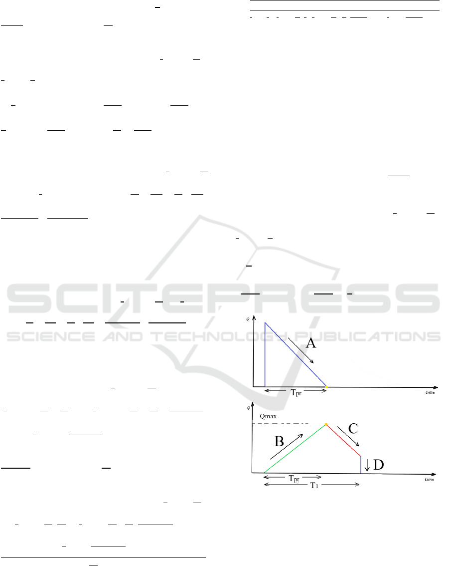
2.3 The Case Tp < Ti
In this case, we assume that the inventory cycle for
imperfect quality items is longer than that of perfect
quality items. Thus, the inventory cycle terminates
when the perfect quality items are depleted. We
assume that the remaining imperfect quality items are
sold in one batch at a lower price of S
d
, where S
p
> S
i
> S
d
. Figures 2a and 2b depict the inventory levels of
the raw material and the finished product.
In this case, T
1
= min {T
p
,T
i
} = T
p
=
(1q)Q
D
i
. Similar
steps followed in the previous case result in:
TC(Q) = K
o
+ K
s
+ CQ + C
p
Q + C
s
Q +
1
2
C
hr
× 
Q
2
P
 +
1
2
C
hf
×

Q
P

2
P  (D
p
+D
i
) +


Q
P

[P
 (D
p
+D
i
)] + Q 

(1-q)Q
D
i

(D
p
+D
i
)

(1-q)Q
D
i

Q
P


(9)
Figure 2a: Raw material inventory (top) Figure 2b: Finished
product inventory (bottom) Tp < Ti.
After T
1
, the remaining products are of imperfect
quality and are to be sold in a single batch at an even
lower selling price S
d
. Thus, the amount of remaining
finished products is T
pr
P − (D
p
+D
i
) T
1
. Hence
ICORES 2020 - 9th International Conference on Operations Research and Enterprise Systems
266

TR(Q) = S
p
qQ + S
i
(qQ)

D
p
D
i

+S
d
Q  
qQ
D
p
 (D
p
+D
i
) 
(10)
The total profit is simply TP(Q) = TR(Q) – TC(Q)
Hence TP(Q) is:
TP(Q)=S
p
qQ+S
i
(qQ)

D
p
D
i

+S
d
Q  
qQ
D
p
 (D
p
+D
i
)  − K
o
− K
s
− CQ − C
p
Q −
C
s
Q −
1
2
C
hr
× 
Q
2
P
 −
1
2
C
hf
× 

Q
P

2
P  (D
p
+D
i
) +


Q
P

[P
 (D
p
+D
i
)] + Q 

(1-q)Q
D
i

(D
p
+D
i
)

(1-q)Q
D
i

Q
P


(11)
The expected total profit is
E[TP(Q)] =
QE(q)+S
i

QD
p
D
i

E(q)
+S
d
Q  Sd
Q
D
p
 (D
p
+D
i
) E(q) − K
o
− K
s
− CQ −
C
p
Q − C
s
Q −
1
2
C
hr
× 
Q
2
P
 −
1
2
C
hf
× 




−






−



+






−




E
(
q
)
−






E
(
q

)

(12)
Using E[TPU(Q)] =
[()]
[]
with T= T
p
=
qQ


, we
have
E[TPU(Q)] =
S

QE
(
q
)
+ S


QD

D

 E
(
q
)
+S

Q  S


Q
D

 D

+D

E
(
q
)
−Ko − Ks − CQ − CpQ − CsQ
−
1
2
C

× 
Q

P
 −
1
2
C

Q
2
× 
2
𝐷

−
𝐷
𝐷


−
1
𝑃
+
2𝐷
𝐷


−
2
𝐷

E
(
q
)
−
𝐷
𝐷


E
(
q

)

Q
𝐷

∙ E[q]
The optimal order quantity is
Q*=

K
o
+K
s
1
2
C
hr
×

1
P

+
1
2
C
hf
×


2
D
i
-
(D
i
+D
p
)
D
i
2
-
1
P
+
2(D
i
+D
p
)
D
i
2
-
2
D
i
∙ E[q] -
(D
i
+D
p
)
D
i
2
∙ E[q
2
]

(13)
3 NUMERICAL EXAMPLES
To illustrate the two models developed in section 2,
consider the situation where a closet manufacturer
sells wooden tables to retailers. The manufacturer
orders wooden boards and assembles them as single
door closets. The percentage of perfect quality boards
ranges between [70% → 90%]. However, after
screening, which is 0.03$ per item, it turns out that
some boards are 180cm and others are 160cm of
height. The 180cm boards are considered of perfect
quality and the 160cm boards are the imperfect
quality. The manufacturer can produce 300 perfect
quality closets per day, and 100 imperfect quality
closets per day, with a production cost of $10 per
product. The purchasing cost is 4$ per wooden board,
and the ordering cost is 1,000$, and the setup cost for
production is $250. The retailers demand 100 units of
180cm closets per day, and 50 units of 160cm closets
per day. Each 180cm closet costs the retailer 450$ and
300$ for the 160cm closets. The holding cost of raw
material is 0.01$ per unit per day and for the finished
products is 0.02$ per unit per day. Find the optimal
number of wooden boards per order Q*, then find the
total profit per cycle. E[q] = 𝜇=
0.7+0.9
2
= 0.8 and E[q
2
]
= Var(q) + (E[q])
2
= 0.00367+0.64= 0.64367. Hence,
Q*= 4,541.6 ≈ 4,542 units and the total profit per unit
time is TPUQ
*
=
TP(Q
*
)
T
=
TP(Q
*
)
qQ
D
p
= 53,013.2$.
Now suppose that the percentage of perfect quality
boards ranges between [60% → 80%]. The
manufacturer can produce 200 perfect quality tables
per day, and 150 imperfect quality tables per day,
with a production cost of $5 per product. The
purchasing cost is 1$ per wooden board, and the
ordering cost is 400$, and the setup cost for
production is $100. The retailers demand 100 units of
3cm thick tables per day, and 50 units of 2cm tables
per day. Each 3cm thick table costs the retailer 30$
and 20$ for the 2cm thick tables. The holding cost of
raw material is 0.01$ per unit per day and for the
finished products is 0.015$ per unit per day. It turned
out that the 3cm thick tables are sold out before the
2cm thick tables. Assume that the manufacturer sells
all the remaining 2cm thick tables at once at a
discounted price of 15$. Then Q* = 3,504.7 ≈ 3,505
units.
4 CONCLUSION
A mathematical function was developed to introduce
an EPQ model that uses both the perfect and
imperfect quality items of raw material in the
production of the finished product. The production
process results in two types of finished products,
perfect and imperfect. A continuous demand is
assumed for both perfect and imperfect quality
finished items. The mathematical model was
formulated for two cases that depend on the length of
the inventory cycles for the perfect and imperfect
quality finished items.
The variability of holding cost is a crucial
A Production Model with Continuous Demand for Imperfect Finished Items Resulting from the Quality of Raw Material
267

requirement, reflecting a realistic assumption in real-
life situations. In fact, in many situations, the holding
cost increases with longer storage periods, as the
extended storage may require more sophisticated, and
thus expensive, storage equipment and conditions. A
case in point could be the storage of food,
pharmaceutical products, and hazardous material that
require certain storage and quality dimensions to
avoid spoilage and/or risk.
The model was validated using a numerical
example. A practical case study will better
demonstrate real-life applications. The model should
also take into consideration the stock type, holding
time, holding cost, demand for perfect quality items,
and demand for imperfect quality items. Moreover,
the models should incorporate the pricing decisions
for both types, as well as the factors influencing the
demand for reach of the types.
Finally, future models should deal with a
coordinated supply chain, consider time value of
money, and incorporate the effect of emission tax.
REFERENCES
Balozian, P., Leidner, D., & Warkentin, M. (2019).
Managers’ and employees’ differing responses to
security approaches. Journal of Computer Information
Systems, 59(3), 197-210.
Balozian, P., & Leidner, D. (2017). Review of IS security
policy compliance: Toward the building blocks of an IS
security theory. ACM SIGMIS Database: the
DATABASE for Advances in Information Systems,
48(3), 11-43.
Bandaly, D. C., & Hassan, H. F. (2019). Postponement
implementation in integrated production and inventory
plan under deterioration effects: a case study of a juice
producer with limited storage capacity. Production
Planning & Control, 1-17.
Bandaly, D., Satir, A., & Shanker, L. (2016). Impact of lead
time variability in supply chain risk
management. International Journal of Production
Economics, 180, 88-100.
Bandaly, D., Satir, A., & Shanker, L. (2014). Integrated
supply chain risk management via operational methods
and financial instruments. International Journal of
Production Research, 52(7), 2007-2025.
Chan, W. M., Ibrahim, R. N., & Lochert, P. B. (2003). A
new EPQ model: integrating lower pricing, rework and
reject situations. Production Planning & Control,
14(7), 588-595.
ElGammal, W., El-Kassar, A. N., & Canaan Messarra, L.
(2018). Corporate ethics, governance and social
responsibility in MENA countries. Management
Decision, 56(1), 273-291.
El-Kassar, A. N. M. (2009). Optimal order quantity for
imperfect quality items. In Allied Academies
International Conference. Academy of Management
Information and Decision Sciences. Proceedings (Vol.
13, No. 1, p. 24). Jordan Whitney Enterprises, Inc.
El-Kassar, A. N., Salameh, M., & Bitar, M. (2012) EPQ
model with imperfect quality raw material.
Mathematica Balkanica, 26, 123-132.
El-Kassar, A. N., Yunis, M., & El-Khalil, R. (2017). The
mediating effects of employee-company identification
on the relationship between ethics, corporate social
responsibility, and organizational citizenship
behavior. Journal of Promotion Management, 23(3),
419-436.
El-Kassar, A. N., & Singh, S. K. (2019). Green innovation
and organizational performance: the influence of big
data and the moderating role of management
commitment and HR practices. Technological
Forecasting and Social Change, 144, 483-498.
El-Khalil, R., & El-Kassar, A. N. (2016). Managing span of
control efficiency and effectiveness: a case
study. Benchmarking: An International Journal, 23(7),
1717-1735.
El-Khalil, R., & El-Kassar, A. N. (2018). Effects of
corporate sustainability practices on performance: the
case of the MENA region. Benchmarking: An
International Journal, 25(5), 1333-1349.
Khan, M., Jaber, M.Y., Guiffrida, A.L., and Zolfaghari, S.
(2011) A review of the extensions of a modified EOQ
model for imperfect quality items, International
Journal of Production Economics 132 (1), 1-12.
Khan, M., and Jaber, M.Y. (2011) Optimal inventory cycle
in a two-stage supply chain incorporating imperfect
items from suppliers, Int. J. Operational Research
10(4), 442–457.
Lamba, K., Singh, S. P., & Mishra, N. (2019). Integrated
decisions for supplier selection and lot-sizing
considering different carbon emission regulations in
Big Data environment. Computers & Industrial
Engineering, 128, 1052-1062.
Pal, S., Mahapatra, G. S., & Samanta, G. P. (2016). A three-
layer supply chain EPQ model for price-and stock-
dependent stochastic demand with imperfect item under
rework. Journal of Uncertainty Analysis and
Applications, 4(1), 10.
Salameh, M. K., & El-Kassar, A. N. (2007, March).
Accounting for the holding cost of raw material in the
production model. In Proceeding of BIMA inaugural
conference (pp. 72-81).
Salameh, M. K., and Jaber, M. Y. (2000) Economic
production quantity model for items with imperfect
quality, International Journal of Production Economics
64, 59–64.
Singh, S. K., & El-Kassar, A. N. (2019). Role of big data
analytics in developing sustainable capabilities. Journal
of cleaner production, 213, 1264-1273.
Singh, S. K., Chen, J., Del Giudice, M., & El-Kassar, A. N.
(2019). Environmental ethics, environmental
performance, and competitive advantage: Role of
environmental training. Technological Forecasting and
Social Change, 146, 203-211.
ICORES 2020 - 9th International Conference on Operations Research and Enterprise Systems
268

Yassine, N. (2016) Joint Probability Distribution and the
Minimum of a Set of Normalized Random Variables,
Procedia - Social and Behavioral Sciences, 230 (12),
235–239.
Yassine, N. & AlSagheer, A. (2017). The optimal solution
of a production model with shortages and raw
materials. Int J Math Comput Methods, 2, 13-18.
Yassine, N. (2018). A sustainable economic production
model: effects of quality and emissions tax from
transportation. Annals of Operations Research, 1-22.
Yassine, N., AlSagheer, A., & Azzam, N. (2018). A
bundling strategy for items with different quality based
on functions involving the minimum of two random
variables. International Journal of Engineering
Business Management, 10, 1-9.
Yassine, N., & El-Rabih, S. (2019, May). Assembling
Components with Probabilistic Lead Times. In IOP
Conference Series: Materials Science and Engineering
(Vol. 521, No. 1, p. 012013).
Yunis, M., Tarhini, A., & Kassar, A. (2018). The role of
ICT and innovation in enhancing organizational
performance: The catalysing effect of corporate
entrepreneurship. Journal of Business Research, 88,
344-356.
Yunis, M., El-Kassar, A. N., & Tarhini, A. (2017). Impact
of ICT-based innovations on organizational
performance: The role of corporate
entrepreneurship. Journal of Enterprise Information
Management, 30(1), 122-141.
A Production Model with Continuous Demand for Imperfect Finished Items Resulting from the Quality of Raw Material
269